\( \DeclareMathOperator{\abs}{abs} \newcommand{\ensuremath}[1]{\mbox{$#1$}} \)
Roulette Curves with Gnu/Linux
1) A Very Complex Roulette: Ellipse Rolling on Ellipse
| (%i2) |
kill
(
all
)
$
define ( fx ( t , af , bf ) , trigsimp ( af · cos ( − t + %pi / 2 ) + %i · bf · sin ( − t + %pi / 2 ) ) ) ; define ( dfx ( t , af , bf ) , diff ( fx ( t , af , bf ) , t ) ) ; |
\[\operatorname{ }\operatorname{fx}\left( t\operatorname{,}\ensuremath{\mathrm{af}}\operatorname{,}\ensuremath{\mathrm{bf}}\right) \operatorname{:=}\ensuremath{\mathrm{af}} \sin{(t)}+i \ensuremath{\mathrm{bf}} \cos{(t)}\]
\[\operatorname{ }\operatorname{dfx}\left( t\operatorname{,}\ensuremath{\mathrm{af}}\operatorname{,}\ensuremath{\mathrm{bf}}\right) \operatorname{:=}\ensuremath{\mathrm{af}} \cos{(t)}-i \ensuremath{\mathrm{bf}} \sin{(t)}\]
| (%i3) | sfx ( t , af , bf ) : = af · elliptic_e ( t , 1 − bf ^ 2 / af ^ 2 ) ; |
\[\operatorname{ }\operatorname{sfx}\left( t\operatorname{,}\ensuremath{\mathrm{af}}\operatorname{,}\ensuremath{\mathrm{bf}}\right) \operatorname{:=}\ensuremath{\mathrm{af}} \operatorname{elliptic\_ e}\left( t\operatorname{,}1-\frac{{{\ensuremath{\mathrm{bf}}}^{2}}}{{{\ensuremath{\mathrm{af}}}^{2}}}\right) \]
| (%i6) |
define
(
ro
(
u
,
ar
,
br
,
cr
)
,
trigexpand
(
trigsimp
(
ar
·
cos
(
u
−
%pi
/
2
)
+
%i
·
br
·
sin
(
u
−
%pi
/
2
)
)
)
+
%i
·
cr
)
;
define ( dro ( u , ar , br ) , diff ( ro ( u , ar , br , cr ) , u ) ) ; sro ( u , ar , br ) : = ar · elliptic_e ( u , 1 − br ^ 2 / ar ^ 2 ) ; |
\[\operatorname{ }\operatorname{ro}\left( u\operatorname{,}\ensuremath{\mathrm{ar}}\operatorname{,}\ensuremath{\mathrm{br}}\operatorname{,}\ensuremath{\mathrm{cr}}\right) \operatorname{:=}\ensuremath{\mathrm{ar}} \sin{(u)}-i \ensuremath{\mathrm{br}} \cos{(u)}+i \ensuremath{\mathrm{cr}}\]
\[\operatorname{ }\operatorname{dro}\left( u\operatorname{,}\ensuremath{\mathrm{ar}}\operatorname{,}\ensuremath{\mathrm{br}}\right) \operatorname{:=}i \ensuremath{\mathrm{br}} \sin{(u)}+\ensuremath{\mathrm{ar}} \cos{(u)}\]
\[\operatorname{ }\operatorname{sro}\left( u\operatorname{,}\ensuremath{\mathrm{ar}}\operatorname{,}\ensuremath{\mathrm{br}}\right) \operatorname{:=}\ensuremath{\mathrm{ar}} \operatorname{elliptic\_ e}\left( u\operatorname{,}1-\frac{{{\ensuremath{\mathrm{br}}}^{2}}}{{{\ensuremath{\mathrm{ar}}}^{2}}}\right) \]
| (%i8) |
load
(
draw
)
$
set_draw_defaults ( xrange = [ − 4 , 4 ] , yrange = [ − 4 , 4 ] , proportional_axes = xy , nticks = 200 , grid = true , background_color = light_yellow , xlabel = "Real Axis" , ylabel = "Imaginary Axis" ) $ |
| (%i14) |
ar
:
1
/
4
$
br
:
1
/
2
$
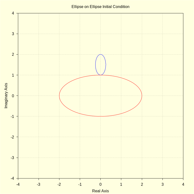
af : 2 $ bf : 1 $ cr : bf + br $ wxdraw2d ( color = blue , parametric ( realpart ( ro ( u , ar , br , cr ) ) , imagpart ( ro ( u , ar , br , cr ) ) , u , 0 , 2 · %pi ) , color = red , parametric ( realpart ( fx ( t , af , bf ) ) , imagpart ( fx ( t , af , bf ) ) , t , 0 , 2 · %pi ) , title = "Ellipse on Ellipse Initial Condition" ) $ |
\[\operatorname{ }\]
We equate arc lengths: af*elliptic_e(t,1-bf^2/af^2) = ar*elliptic_e(u,1-br^2/ar^2).
The inversion of an elliptic integral of the second kind is not possible (aside from very complex extraordinary methods) and hence we invert the function numerically.
| (%i15) | load ( newton1 ) $ |
| (%i22) |
kill
(
t
,
u
)
$
ar : 1 / 4 $ br : 1 / 2 $ af : 2 $ bf : 1 $ t : 4 . 0 ; ut : newton ( sro ( u , ar , br ) − sfx ( t , af , bf ) , u , t , 1e-10 ) ; |
\[\operatorname{(t) }4.0\]
\[\operatorname{(ut) }16.76796630164899\]
| (%i24) |
sfx
(
t
,
af
,
bf
)
;
sro ( ut , ar , br ) ; |
\[\operatorname{ }6.413548139974258\]
\[\operatorname{ }6.413548139993162\]
| (%i27) |
kill
(
t
,
u
,
af
,
bf
,
ar
,
br
)
$
depends ( u , t ) $ define ( dudt ( t , u , af , bf , ar , br ) , rhs ( solve ( factor ( cabs ( diff ( ro ( u , ar , br , cr ) , t ) ) ) = cabs ( dfx ( t , af , bf ) ) , diff ( u , t ) ) [ 1 ] ) ) ; |
\[\operatorname{ }\operatorname{dudt}\left( t\operatorname{,}u\operatorname{,}\ensuremath{\mathrm{af}}\operatorname{,}\ensuremath{\mathrm{bf}}\operatorname{,}\ensuremath{\mathrm{ar}}\operatorname{,}\ensuremath{\mathrm{br}}\right) \operatorname{:=}\frac{\sqrt{{{\ensuremath{\mathrm{bf}}}^{2}} {{\sin{(t)}}^{2}}+{{\ensuremath{\mathrm{af}}}^{2}} {{\cos{(t)}}^{2}}}}{\sqrt{{{\ensuremath{\mathrm{br}}}^{2}} {{\sin{(u)}}^{2}}+{{\ensuremath{\mathrm{ar}}}^{2}} {{\cos{(u)}}^{2}}}}\]
2) Generate the Roulette
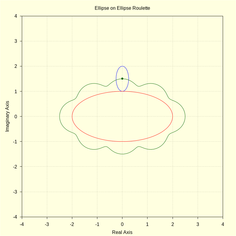
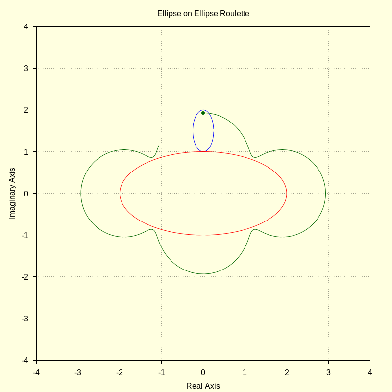
For the first example, we select p, the generating point, to be at the center of the rolling ellipse.
| (%i28) | M : zeromatrix ( 600 , 2 ) $ |
| (%i34) |
kill
(
t
,
u
,
af
,
bf
,
ar
,
br
)
$
ar : 1 / 4 $ br : 1 / 2 $ af : 2 $ bf : 1 $ p : %i · ( bf + br ) ; |
\[\operatorname{(p) }\frac{3 i}{2}\]
| (%i37) |
t
:
0
$
tinc
:
0
.
015
$
for i : 1 thru 600 step 1 do ( u : newton ( sro ( uu , ar , br ) − sfx ( t , af , bf ) , uu , t , 1e-10 ) , roul : fx ( t , af , bf ) − ( ro ( u , ar , br , ( br + bf ) ) − p ) · dfx ( t , af , bf ) / ( dro ( u , ar , br ) · dudt ( t , u , af , bf , ar , br ) ) , M [ i , 1 ] : float ( realpart ( roul ) ) , M [ i , 2 ] : float ( imagpart ( roul ) ) , t : t + tinc ) $ |
| (%i40) |
kill
(
u
,
t
)
$
wxdraw2d ( color = blue , parametric ( realpart ( ro ( u , ar , br , ( br + bf ) ) ) , imagpart ( ro ( u , ar , br , ( br + bf ) ) ) , u , 0 , 2 · %pi ) , color = red , parametric ( realpart ( fx ( t , af , bf ) ) , imagpart ( fx ( t , af , bf ) ) , t , 0 , 2 · %pi ) , color = darkgreen , point_size = 1 , point_type = 7 , points ( [ [ realpart ( p ) , imagpart ( p ) ] ] ) , point_type = 0 , points_joined = true , points ( M ) , title = "Ellipse on Ellipse Roulette" ) $ |
\[\operatorname{ }\]
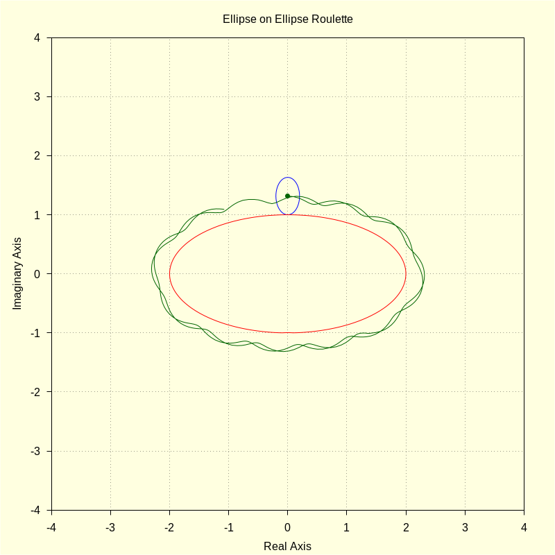
The next example shows an incommensurate case.
| (%i46) |
kill
(
t
,
u
,
af
,
bf
,
ar
,
br
)
$
ar : 1 / 5 $ br : 1 / sqrt ( 10 ) $ af : 2 $ bf : 1 $ p : %i · ( bf + br ) ; |
\[\operatorname{(p) }\left( \frac{1}{\sqrt{10}}+1\right) i\]
| (%i49) |
t
:
0
$
tinc
:
0
.
02
$
for i : 1 thru 600 step 1 do ( u : newton ( sro ( uu , ar , br ) − sfx ( t , af , bf ) , uu , t , 1e-10 ) , roul : fx ( t , af , bf ) − ( ro ( u , ar , br , ( br + bf ) ) − p ) · dfx ( t , af , bf ) / ( dro ( u , ar , br ) · dudt ( t , u , af , bf , ar , br ) ) , M [ i , 1 ] : float ( realpart ( roul ) ) , M [ i , 2 ] : float ( imagpart ( roul ) ) , t : t + tinc ) $ |
| (%i52) |
kill
(
u
,
t
)
$
wxdraw2d ( color = blue , parametric ( realpart ( ro ( u , ar , br , ( br + bf ) ) ) , imagpart ( ro ( u , ar , br , ( br + bf ) ) ) , u , 0 , 2 · %pi ) , color = red , parametric ( realpart ( fx ( t , af , bf ) ) , imagpart ( fx ( t , af , bf ) ) , t , 0 , 2 · %pi ) , color = darkgreen , point_size = 1 , point_type = 7 , points ( [ [ realpart ( p ) , imagpart ( p ) ] ] ) , point_type = 0 , points_joined = true , points ( M ) , title = "Ellipse on Ellipse Roulette" ) $ |
\[\operatorname{ }\]
| (%i58) |
kill
(
t
,
u
,
af
,
bf
,
ar
,
br
)
$
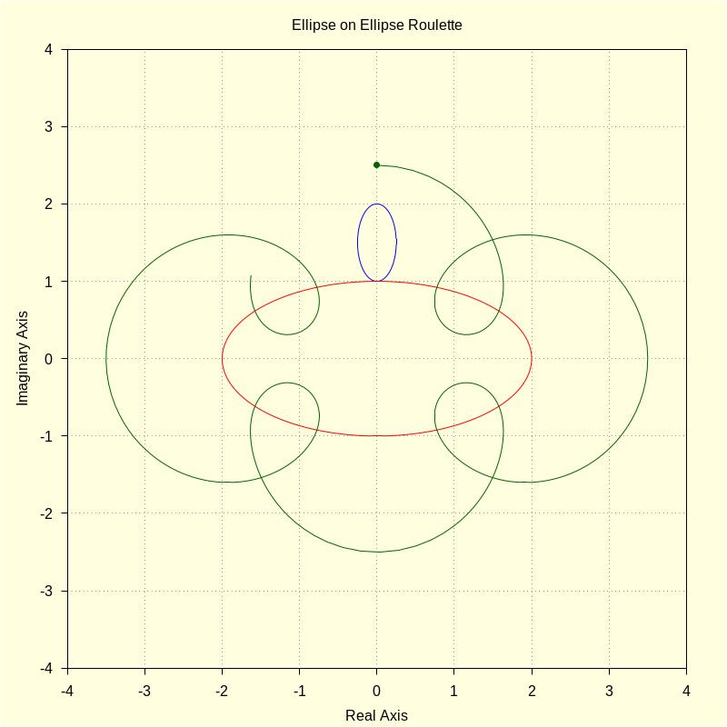
ar : 1 / 4 $ br : 1 / 2 $ af : 2 $ bf : 1 $ p : %i · ( bf + br + 1 ) ; |
\[\operatorname{(p) }\frac{5 i}{2}\]
| (%i61) |
t
:
0
$
tinc
:
0
.
01
$
for i : 1 thru 600 step 1 do ( u : newton ( sro ( uu , ar , br ) − sfx ( t , af , bf ) , uu , t , 1e-10 ) , roul : fx ( t , af , bf ) − ( ro ( u , ar , br , ( br + bf ) ) − p ) · dfx ( t , af , bf ) / ( dro ( u , ar , br ) · dudt ( t , u , af , bf , ar , br ) ) , M [ i , 1 ] : float ( realpart ( roul ) ) , M [ i , 2 ] : float ( imagpart ( roul ) ) , t : t + tinc ) $ |
| (%i64) |
kill
(
u
,
t
)
$
wxdraw2d ( color = blue , parametric ( realpart ( ro ( u , ar , br , ( br + bf ) ) ) , imagpart ( ro ( u , ar , br , ( br + bf ) ) ) , u , 0 , 2 · %pi ) , color = red , parametric ( realpart ( fx ( t , af , bf ) ) , imagpart ( fx ( t , af , bf ) ) , t , 0 , 2 · %pi ) , color = darkgreen , point_size = 1 , point_type = 7 , points ( [ [ realpart ( p ) , imagpart ( p ) ] ] ) , point_type = 0 , points_joined = true , points ( M ) , title = "Ellipse on Ellipse Roulette" ) $ |
\[\operatorname{ }\]
| (%i70) |
kill
(
t
,
u
,
af
,
bf
,
ar
,
br
)
$
ar : 1 / 4 $ br : 1 / 2 $ af : 2 $ bf : 1 $ p : %i · ( bf + br + sqrt ( br ^ 2 − ar ^ 2 ) ) ; |
\[\operatorname{(p) }\left( \frac{\sqrt{3}}{4}+\frac{3}{2}\right) i\]
| (%i73) |
t
:
0
$
tinc
:
0
.
01
$
for i : 1 thru 600 step 1 do ( u : newton ( sro ( uu , ar , br ) − sfx ( t , af , bf ) , uu , t , 1e-10 ) , roul : fx ( t , af , bf ) − ( ro ( u , ar , br , ( br + bf ) ) − p ) · dfx ( t , af , bf ) / ( dro ( u , ar , br ) · dudt ( t , u , af , bf , ar , br ) ) , M [ i , 1 ] : float ( realpart ( roul ) ) , M [ i , 2 ] : float ( imagpart ( roul ) ) , t : t + tinc ) $ |
| (%i76) |
kill
(
u
,
t
)
$
wxdraw2d ( color = blue , parametric ( realpart ( ro ( u , ar , br , ( br + bf ) ) ) , imagpart ( ro ( u , ar , br , ( br + bf ) ) ) , u , 0 , 2 · %pi ) , color = red , parametric ( realpart ( fx ( t , af , bf ) ) , imagpart ( fx ( t , af , bf ) ) , t , 0 , 2 · %pi ) , color = darkgreen , point_size = 1 , point_type = 7 , points ( [ [ realpart ( p ) , imagpart ( p ) ] ] ) , point_type = 0 , points_joined = true , points ( M ) , title = "Ellipse on Ellipse Roulette" ) $ |
\[\operatorname{ }\]
3) Epilogue
Created with
wxMaxima.
Modified and embedded by L.A.P.
First, we define the fixed curve, which is an ellipse in standard form centered at the origin of the complex plane, and its derivative. The variables af, bf denote those of the fixed curve, while the rolling is defined using ar, br.
The rolling curve, sitting atop the fixed ellipse, must properly map onto the fixed ellipse. This necessitates for the fixed ellipse a clockwise rotation beginning at the point 0, i * b: