The Web Site of L.A.P.

Roulette Curves with GNU/Linux

1) Introduction

A roulette is the locus of a point on, or off, a curve, called the rolling curve, that rolls without slipping along another, fixed curve. The patterns produced by such rolling can be appealing aesthetically, but, to me, the challenge of producing such roulettes is the primary allure. In this series of articles I will tackle some of the more demanding roulettes using the excellent computer algebra tools on GNU/Linux, namely Maxima and its graphical front end wxMaxima.

We will be using Maxima/wxMaxima throughout to derive equations and to plot results. Unfortunately, these articles cannot be a primer to Maxima and the reader should have some familiarity with Maxima syntax, which is rather straightforward. The reader also should be familiar with the concepts of basic Calculus, Analytical Geometry, and Trigonometry.

2) Overview of Roulette Mathematics

Roulettes will be represented with parameterization using complex numbers rather than the usual Cartesian coordinates. The reason for this is that the complex plane allows for more efficient derivations. Rotations, for example, are accomplished with simple complex multiplication rather that the use of cumbersome matrices.

Any curve in the complex plane is described using a real parameter, t.

Z(t) = f(t) + i * g(t)

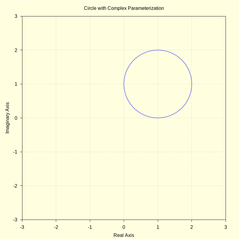
A circle, with center at xc, i * yc is:

(%i1)

kill ( all ) $

(%i1)

circ ( t , R , xc , yc ) : = R · cos ( t ) + %i · R · sin ( t ) + xc + %i · yc ;

\[\operatorname{ }\operatorname{circ}\left( t\operatorname{,}R\operatorname{,}\ensuremath{\mathrm{xc}}\operatorname{,}\ensuremath{\mathrm{yc}}\right) \operatorname{:=}R \cos{(t)}+i R \sin{(t)}+\ensuremath{\mathrm{xc}}+i \ensuremath{\mathrm{yc}}\]

Complex parameterized curves are easily plotted:

(%i3)

load ( draw ) $ set_draw_defaults ( xrange = [ − 3 , 3 ] , yrange = [ − 3 , 3 ] , proportional_axes = xy , grid = true , nticks = 400 ,
background_color = light_yellow , xlabel = "Real Axis" , ylabel = "Imaginary Axis" ) $

(%i8)

kill ( t ) $ R : 1 $ xc : 1 $ yc : 1 $
wxdraw2d ( parametric ( realpart ( circ ( t , R , xc , yc ) ) , imagpart ( circ ( t , R , xc , yc ) ) , t , 0 , 2 · %pi ) ,
title = "Circle with Complex Parameterization" ) $

\[\operatorname{ }\]

We consider two curves: a fixed curve, fx(t), and a rolling curve, ro(u). The two curves are defined using different parameters, t and u.

To ensure a no-slip condition, the arc-lengths of both curves must be equal as the parameters t and u evolve. This condition is established by equating the two expressions for arc-length, which we will call sfx(t) and sro(u), and then solving for u as a function of t: u = u(t). If the solution cannot be obtained analytically then a numerical solution is found for each value of t as the roulette is generated.

Initially, the two curves are in contact with fx(0) = ro(0) and fx'(0) = ro'(0), that is the functions and their first derivatives are equal.

Also, the magnitudes of the first derivatives must be equal at every point:
|fx'(t)| = |ro'(u(t))|.

If an analytical u(t) can't be found then a value for the first derivative of the rolling curve, ro'(u(t)), must be determined at each point. The later examples will show how this done.

Given all the above conditions, the roulette equation is:

roul(t) = fx(t) + (p - ro(u(t))) * fx'(t)/ro'(t)

The complex point, p, actually generates the roulette and it can be located on the rolling curve or anywhere else. We can view the plane containing the rolling curve, as well as the point p that is located anywhere, as actually rolling (or rotating) and carrying both the rolling curve and p with it.

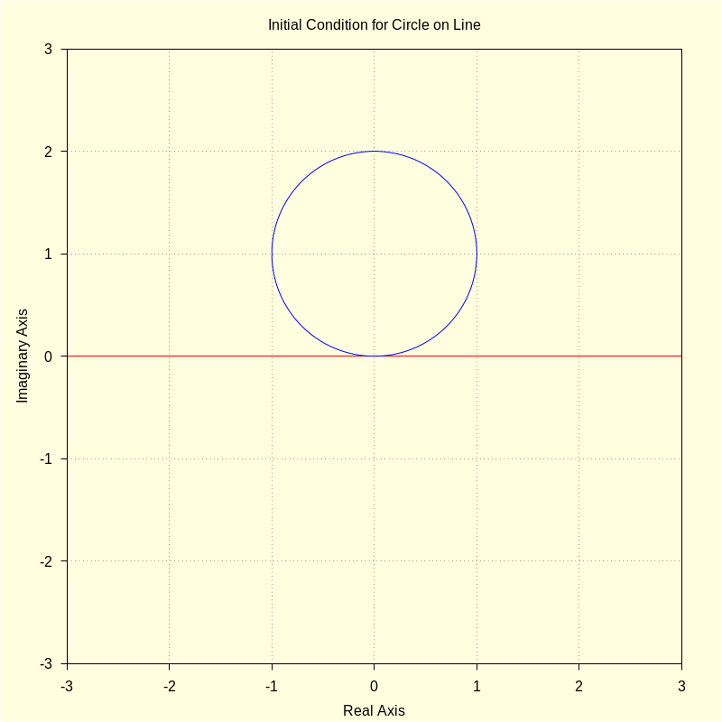
To make all the above clear, we will consider perhaps the simplest roulette, that of a circle rolling on a line, with the line being the x-axis (or real axis) and the circle being located initially at the complex point 0, i * R.

3) A Simple Roulette: Circle Rolling on Line

We allow the rolling curve, ro(u), to roll to right with a clockwise rotation starting at 0, 0 and this necessitates the following parameterization.

(%i1)

kill ( all ) $
define ( ro ( u , R , xc , yc ) , trigsimp ( R · ( cos ( u − %pi / 2 ) + %i · sin ( u − %pi / 2 ) ) + xc + %i · yc ) ) ;

\[\operatorname{ }\operatorname{ro}\left( u\operatorname{,}R\operatorname{,}\ensuremath{\mathrm{xc}}\operatorname{,}\ensuremath{\mathrm{yc}}\right) \operatorname{:=}i \ensuremath{\mathrm{yc}}+\ensuremath{\mathrm{xc}}+R \sin{(u)}-i R \cos{(u)}\]

Now come the expressions for the derivative, dro(u), and arc-length, sro(u), of the rolling curve.

(%i4)

assume ( R > 0 , u > = 0 ) $
define ( dro ( u , R ) , diff ( ro ( u , R , xc , yc ) , u ) ) ;
define ( sro ( u , R ) , integrate ( cabs ( dro ( u , R ) ) , u ) ) ;

\[\operatorname{ }\operatorname{dro}\left( u\operatorname{,}R\right) \operatorname{:=}i R \sin{(u)}+R \cos{(u)}\]

\[\operatorname{ }\operatorname{sro}\left( u\operatorname{,}R\right) \operatorname{:=}R u\]

The fixed curve, fx(t), is the real axis (x-axis).

(%i5)

fx ( t ) : = t + %i · 0 ;

\[\operatorname{ }\operatorname{fx}(t)\operatorname{:=}t+i 0\]

Now come the expressions for the derivative, dfx(t), and arc-length, sfx(t), of the fixed curve.

(%i7)

define ( dfx ( t ) , diff ( fx ( t ) , t ) ) ;
define ( sfx ( t ) , integrate ( cabs ( dfx ( t ) ) , t ) ) ;

\[\operatorname{ }\operatorname{dfx}(t)\operatorname{:=}1\]

\[\operatorname{ }\operatorname{sfx}(t)\operatorname{:=}t\]

A plot of the initial conditions for the roulette generation

(%i11)

R : 1 $ xc : 0 $ yc : 1 $
wxdraw2d ( color = red , parametric ( realpart ( fx ( t ) ) , imagpart ( fx ( t ) ) , t , − 3 , 3 ) , color = blue , parametric ( realpart ( ro ( u , R , xc , yc ) ) ,
imagpart ( ro ( u , R , xc , yc ) ) , u , 0 , 2 · %pi ) ,
title = "Initial Conditions for Circle on Line"
) $

\[\operatorname{ }\]

Now we equate the equations for arc-length and then solve for u = u(t). (In this case, this is easy. For later roulette examples it becomes much more difficult.)

(%i13)

kill ( t , u , R , xc , yc ) $
define ( ut ( t , R ) , rhs ( solve ( sfx ( t ) = sro ( u , R ) , u ) [ 1 ] ) ) ;

\[\operatorname{ }\operatorname{ut}\left( t\operatorname{,}R\right) \operatorname{:=}\frac{t}{R}\]

For the no-slip condition, the parameter for the rolling curve must be u(t) = t / R. We must now re-define the rolling curve function in terms of u(t) by substitution into into the original expression.

(%i16)

define ( ro ( t , R , xc , yc ) , trigsimp ( R · ( cos ( ut ( t , R ) − %pi / 2 ) + %i · sin ( ut ( t , R ) − %pi / 2 ) ) + xc + %i · yc ) ) ;
assume ( R > 0 , u > = 0 ) $
define ( dro ( t , R ) , diff ( ro ( t , R , xc , yc ) , t ) ) ;

\[\operatorname{ }\operatorname{ro}\left( t\operatorname{,}R\operatorname{,}\ensuremath{\mathrm{xc}}\operatorname{,}\ensuremath{\mathrm{yc}}\right) \operatorname{:=}i \ensuremath{\mathrm{yc}}+\ensuremath{\mathrm{xc}}+R \sin{\left( \frac{t}{R}\right) }-i R \cos{\left( \frac{t}{R}\right) }\]

\[\operatorname{ }\operatorname{dro}\left( t\operatorname{,}R\right) \operatorname{:=}i \sin{\left( \frac{t}{R}\right) }+\cos{\left( \frac{t}{R}\right) }\]

Let's check if the initial conditions, as stated above, apply.

(%i20)

xc : 0 $ yc : R $
fx ( 0 ) ;
ro ( 0 , R , xc , yc ) ;

\[\operatorname{ }0\]

OK. They are equal.

Do the first derivatives at t = 0 equal? Note that we want dy/dx and thus we take the ratio (dy/dt) / (dx/dt).

(%i22)

imagpart ( dfx ( 0 ) ) / realpart ( dfx ( 0 ) ) ;
imagpart ( dro ( 0 , R ) ) / realpart ( dro ( 0 , R ) ) ;

\[\operatorname{ }0\]

OK. They are equal.

Are the magnitudes of the first derivatives equal for all t?

(%i24)

cabs ( dfx ( t ) ) ;
trigsimp ( cabs ( dro ( t , R ) ) ) ;

\[\operatorname{ }1\]

OK. They are equal.

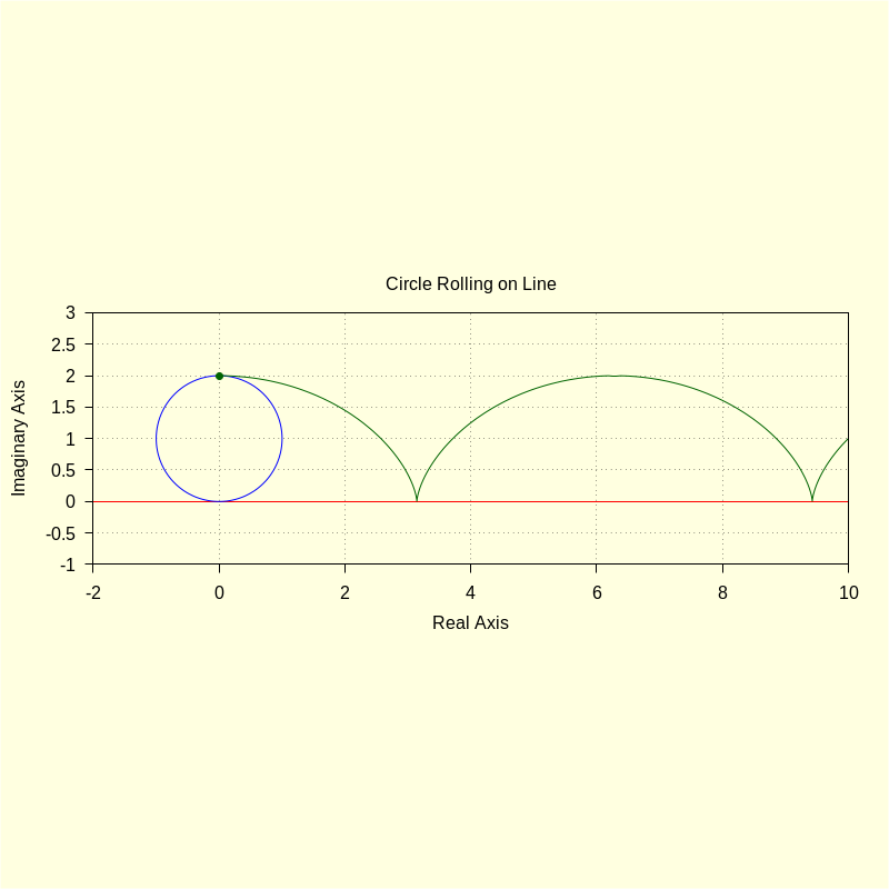
4) Generating the Roulette

All of our functions being defined, we select a generating point, p, and then produce the roulette.

(%i28)

p : 0 + %i · 2 ; R : 1 $ ; xc : 0 $ yc : R $

\[\operatorname{(p) }2 i\]

(%i29)

define ( roul ( t ) , fx ( t ) + ( p − ro ( t , R , xc , yc ) ) · dfx ( t ) / dro ( t , R ) ) ;

\[\operatorname{ }\operatorname{roul}(t)\operatorname{:=}\frac{-\sin{(t)}+i \cos{(t)}+i}{i \sin{(t)}+\cos{(t)}}+t\]

(%i30)

wxdraw2d ( xrange = [ − 2 , 10 ] , yrange = [ − 1 , 3 ] ,
   color = blue , parametric ( realpart ( fx ( t ) ) , imagpart ( fx ( t ) ) , t , − 2 , 10 ) ,
   color = red , parametric ( realpart ( ro ( t , R , xc , yc ) ) , imagpart ( ro ( t , R , xc , yc ) ) , t , 0 , 2 · %pi ) ,
   color = darkgreen , parametric ( realpart ( roul ( t ) ) , imagpart ( roul ( t ) ) , t , 0 , 4 · %pi ) ,
   point_type = 7 , points [ [ realpart ( p ) ] , [ imagpart ( p ) ] ] ,
   title = "Circle Rolling on Line"
) $

\[\operatorname{ }\]

In this case, the roulette equation defined above, simplifies to the familiar cycloid.

(%i32)

trigsimp ( realpart ( roul ( t ) ) ) ;
trigsimp ( imagpart ( roul ( t ) ) ) ;

\[\operatorname{ }\sin{(t)}+t\]

\[\operatorname{ }\cos{(t)}+1\]

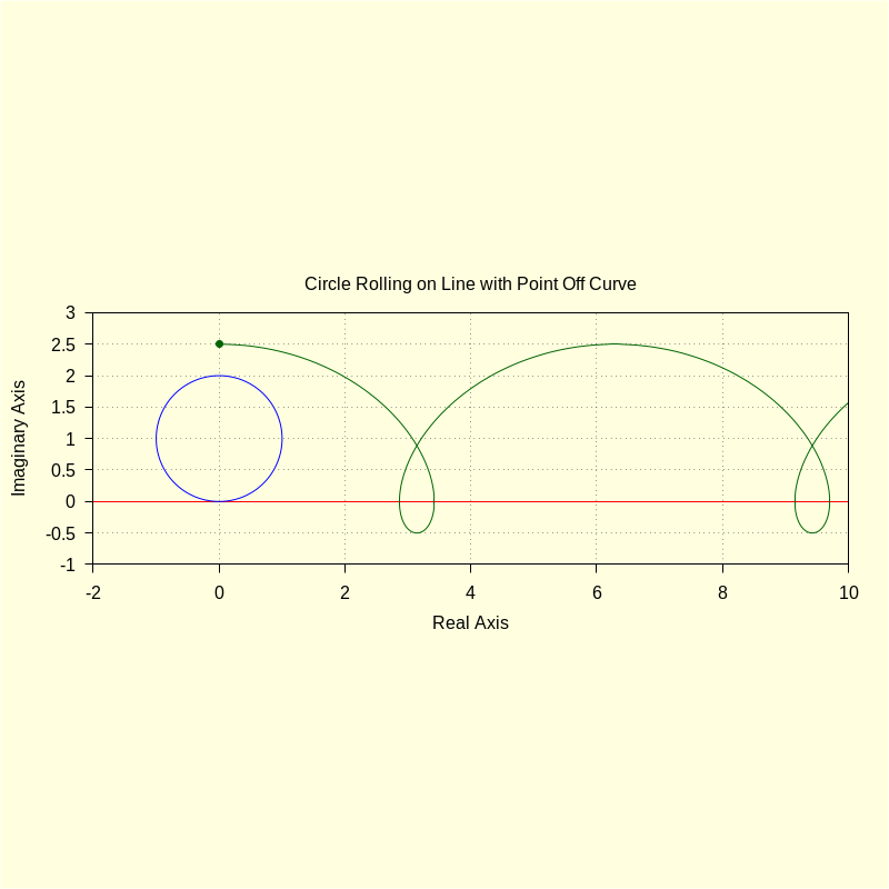
But point p need not be on the actual rolling curve. Let us select p = -5/2 * R * i

(%i37)

R : 1 $ ; xc : 0 $ yc : R $
p : %i · R · 5 / 2 ;
define ( roul ( t ) , fx ( t ) + ( p − ro ( t , R , xc , yc ) ) · dfx ( t ) / dro ( t , R ) ) ;

\[\operatorname{(p) }\frac{5 i}{2}\]

\[\operatorname{ }\operatorname{roul}(t)\operatorname{:=}\frac{-\sin{(t)}+i \cos{(t)}+\frac{3 i}{2}}{i \sin{(t)}+\cos{(t)}}+t\]

(%i38)

\[\operatorname{ }\]

Let's place p at the center of the circle

(%i43)

R : 1 $ ; xc : 0 $ yc : R $
p : %i ;
define ( roul ( t ) , fx ( t ) + ( p − ro ( t , R , xc , yc ) ) · dfx ( t ) / dro ( t , R ) ) ;

\[\operatorname{(p) }i\]

\[\operatorname{ }\operatorname{roul}(t)\operatorname{:=}\frac{i \cos{(t)}-\sin{(t)}}{i \sin{(t)}+\cos{(t)}}+t\]

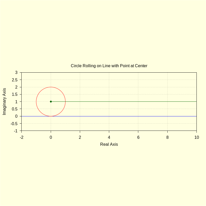
(%i44)

wxdraw2d ( xrange = [ − 2 , 10 ] , yrange = [ − 1 , 3 ] ,
   color = blue , parametric ( realpart ( fx ( t ) ) , imagpart ( fx ( t ) ) , t , − 2 , 10 ) ,
   color = red , parametric ( realpart ( ro ( u , R , xc , yc ) ) , imagpart ( ro ( u , R , xc , yc ) ) , u , 0 , 2 · %pi ) ,
   color = darkgreen , parametric ( realpart ( roul ( t ) ) , imagpart ( roul ( t ) ) , t , 0 , 4 · %pi ) ,
   point_type = 7 , points [ [ realpart ( p ) ] , [ imagpart ( p ) ] ] ,
   title = "Circle Rolling on Line with Point at Center"
) $

\[\operatorname{ }\]

Can we obtain a general expression for this roulette?

(%i48)

kill ( t , R , xc , yc , p ) $
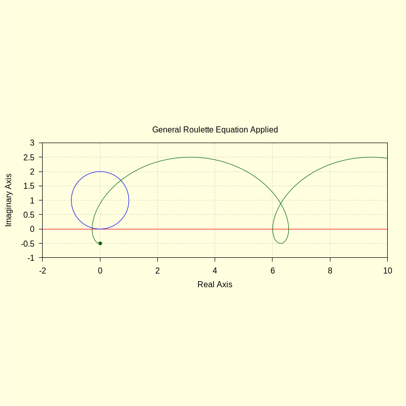
define ( roul ( t ) , fx ( t ) + ( p − ro ( t , R , xc , yc ) ) · dfx ( t ) / dro ( t , R ) ) ;
trigsimp ( realpart ( roul ( t ) ) ) ;
trigsimp ( imagpart ( roul ( t ) ) ) ;

\[\operatorname{ }\operatorname{roul}(t)\operatorname{:=}\frac{-i \ensuremath{\mathrm{yc}}-\ensuremath{\mathrm{xc}}-R \sin{\left( \frac{t}{R}\right) }+i R \cos{\left( \frac{t}{R}\right) }+p}{i \sin{\left( \frac{t}{R}\right) }+\cos{\left( \frac{t}{R}\right) }}+t\]

\[\operatorname{ }-\sin{\left( \frac{t}{R}\right) } \ensuremath{\mathrm{yc}}-\cos{\left( \frac{t}{R}\right) } \ensuremath{\mathrm{xc}}+p \cos{\left( \frac{t}{R}\right) }+t\]

\[\operatorname{ }-\cos{\left( \frac{t}{R}\right) } \ensuremath{\mathrm{yc}}+\sin{\left( \frac{t}{R}\right) } \ensuremath{\mathrm{xc}}-p \sin{\left( \frac{t}{R}\right) }+R\]

Let's plot this again for R = 1 and p = 0, -i/2

(%i53)

R : 1 $ xc : 0 $ yc : R $
p : − %i · 1 / 2 ;
wxdraw2d ( xrange = [ − 2 , 10 ] , yrange = [ − 1 , 3 ] ,
   color = blue , parametric ( realpart ( fx ( t ) ) , imagpart ( fx ( t ) ) , t , − 2 , 10 ) ,
   color = red , parametric ( realpart ( ro ( u , R , xc , yc ) ) , imagpart ( ro ( u , R , xc , yc ) ) , u , 0 , 2 · %pi ) ,
   color = darkgreen , parametric ( realpart ( roul ( t ) ) , imagpart ( roul ( t ) ) , t , 0 , 4 · %pi ) ,
   point_type = 7 , points [ [ realpart ( p ) ] , [ imagpart ( p ) ] ] ,
   title = "General Roulette Equation Applied"
) $

\[\operatorname{(p) }-\frac{i}{2}\]

\[\operatorname{ }\]

So this general equation can be used to produce all such roulettes.

5) Parting Comments

Although this roulette of a circle rolling on a line is quite simple, it illustrates the basic method that will be used for more mathematically, if not visually, complex roulettes.

Maxima/wxMaxima will assist in eliminating the burdensome derivations and allow us to concentrate solely on the mathematical concepts.

Analytical equations of the roulettes are not always possible, but numerical routines, also provided by Maxima/wxMaxima, will allow us to easily visualize any roulette.

The subsequent examples will assume familiarity with the methods of this introduction and we will not be as detailed in the development as we are here.

Created with wxMaxima.
Modified and embedded by L.A.P.