\( \DeclareMathOperator{\abs}{abs} \newcommand{\ensuremath}[1]{\mbox{$#1$}} \)
Roulette Curves with GNU/Linux
1) We now consider a complex roulette that requires a numerical rather than an analytical solution: Ellipse Rolling on Line
| (%i3) |
fx
(
t
)
:
=
t
+
%i
·
0
;
define ( dfx ( t ) , diff ( fx ( t ) , t ) ) ; define ( sfx ( t ) , integrate ( cabs ( dfx ( t ) ) , t ) ) ; |
\[\operatorname{ }\operatorname{fx}(t)\operatorname{:=}t+i 0\]
\[\operatorname{ }\operatorname{dfx}(t)\operatorname{:=}1\]
\[\operatorname{ }\operatorname{sfx}(t)\operatorname{:=}t\]
The mapping has to start from 0, 0 (not b, a) hence the parameter u is shifted back by %pi/2.
We also derive the first derivative and the arc length.
| (%i6) |
define
(
ro
(
u
,
a
,
b
)
,
ev
(
trigsimp
(
b
·
cos
(
u
−
%pi
/
2
)
+
%i
·
a
·
sin
(
u
−
%pi
/
2
)
+
%i
·
a
)
)
)
;
define ( dro ( u , a , b ) , diff ( ro ( u , a , b ) , u ) ) ; define ( sro ( u , a , b ) , integrate ( cabs ( dro ( u , a , b ) ) , u ) ) ; |
\[\operatorname{ }\operatorname{ro}\left( u\operatorname{,}a\operatorname{,}b\right) \operatorname{:=}b \sin{(u)}-i a \cos{(u)}+i a\]
\[\operatorname{ }\operatorname{dro}\left( u\operatorname{,}a\operatorname{,}b\right) \operatorname{:=}i a \sin{(u)}+b \cos{(u)}\]
\[\operatorname{ }\operatorname{sro}\left( u\operatorname{,}a\operatorname{,}b\right) \operatorname{:=}\int {\left. \sqrt{{{a}^{2}} {{\sin{(u)}}^{2}}+{{b}^{2}} {{\cos{(u)}}^{2}}}du\right.}\]
2) A Plot Of The Intitial Condition
| (%i8) |
load
(
draw
)
$
set_draw_defaults ( grid = true , nticks = 200 , background_color = light_yellow , proportional_axes = xy , xlabel = "Real Axis" , ylabel = "Imaginary Axis" ) $ |
| (%i11) |
a
:
2
;
b
:
1
;
wxdraw2d ( xrange = [ − 2 , 10 ] , yrange = [ − 2 , 10 ] , color = red , parametric ( realpart ( fx ( t ) ) , imagpart ( fx ( t ) ) , t , − 2 , 10 ) , color = blue , parametric ( realpart ( ro ( u , a , b ) ) , imagpart ( ro ( u , a , b ) ) , u , 0 , 2 · %pi ) , title = "Ellipse on Line Initial Condition" ) $ |
\[\operatorname{(a) }2\]
\[\operatorname{(b) }1\]
\[\operatorname{ }\]

3) Determine The Relation Between Arc Length Parameters
| (%i12) | kill ( a , b , t , u ) $ |
| (%i13) | sro ( u , a , b ) : = b · elliptic_e ( u , 1 − a ^ 2 / b ^ 2 ) ; |
\[\operatorname{ }\operatorname{sro}\left( u\operatorname{,}a\operatorname{,}b\right) \operatorname{:=}b \operatorname{elliptic\_ e}\left( u\operatorname{,}1-\frac{{{a}^{2}}}{{{b}^{2}}}\right) \]
In Maxima, we have a choice of using either "find_root()" or "newton()" as solvers but we'll use both for this example.
| (%i14) | load ( newton1 ) $ |
First, we find u for a given t using both solvers.
| (%i19) |
t
:
9
$
a
:
2
$
b
:
1
$
u1 : root1 : find_root ( b · elliptic_e ( u , 1 − a ^ 2 / b ^ 2 ) = t , u , 0 , 10 ) ; u2 : root2 : newton ( b · elliptic_e ( u , 1 − a ^ 2 / b ^ 2 ) − t , u , t , 1e-10 ) ; |
\[\operatorname{(u1) }5.683783113001842\]
\[\operatorname{(u2) }5.68378311299735\]
| (%i21) |
b
·
elliptic_e
(
u1
,
1
−
a
^
2
/
b
^
2
)
;
b · elliptic_e ( u2 , 1 − a ^ 2 / b ^ 2 ) ; |
\[\operatorname{ }9.0\]
\[\operatorname{ }8.99999999999372\]
| (%i22) | kill ( t , u , a , b , u1 , u2 ) $ |
The magnitudes, cabs(), of the derivatives of the fixed curve and the rolling curve must be equal for t > 0. This gives a way to find dro() at each step.
We find d/dt [ro(u)] and equate that to sfx(t) and then solve for du/dt. This provides a factor, du/dt, to determine dro(t) at each step. The following illustrates this method.
| (%i25) |
depends
(
u
,
t
)
$
assume ( u > = 0 , t > = 0 ) $ magdro : factor ( cabs ( diff ( ro ( u , a , b ) , t ) ) ) ; |
\[\operatorname{(magdro) }\sqrt{{{a}^{2}} {{\sin{(u)}}^{2}}+{{b}^{2}} {{\cos{(u)}}^{2}}} \left| \frac{d}{d t} u\right| \]
| (%i26) | magdfx : cabs ( dfx ( t ) ) ; |
\[\operatorname{(magdfx) }1\]
| (%i27) | define ( dudt ( u , a , b ) , rhs ( solve ( magdro = magdfx , diff ( u , t ) ) [ 1 ] ) ) ; |
\[\operatorname{ }\operatorname{dudt}\left( u\operatorname{,}a\operatorname{,}b\right) \operatorname{:=}\frac{1}{\sqrt{{{a}^{2}} {{\sin{(u)}}^{2}}+{{b}^{2}} {{\cos{(u)}}^{2}}}}\]
4) Generate Some Roulettes
| (%i28) | kill ( t , u , a , b , p ) $ |
| (%i29) | M : zeromatrix ( 400 , 2 ) $ |
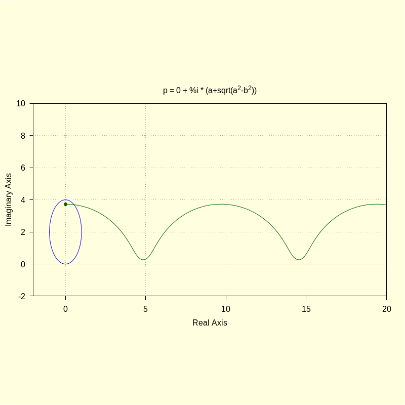
The generating point, p, is set as the upper focus of the ellipse.
| (%i36) |
a
:
2
$
b
:
1
$
p : %i · ( a + sqrt ( a ^ 2 − b ^ 2 ) ) ; t : 0 $ tinc : 0 . 05 $ e : 1 − a ^ 2 / b ^ 2 $ for i : 1 thru 400 step 1 do ( u : newton ( b · elliptic_e ( uu , e ) − t , uu , t , 1e-10 ) , roul : fx ( t ) − ( ro ( u , a , b ) − p ) · dfx ( t ) / ( dro ( u , a , b ) · dudt ( u , a , b ) ) , M [ i , 1 ] : float ( realpart ( roul ) ) , M [ i , 2 ] : float ( imagpart ( roul ) ) , t : t + tinc ) $ |
\[\operatorname{(p) }\left( \sqrt{3}+2\right) i\]
| (%i38) |
kill
(
t
,
u
)
$
wxdraw2d ( xrange = [ − 2 , 20 ] , yrange = [ − 2 , 10 ] , color = blue , parametric ( realpart ( ro ( t , a , b ) ) , imagpart ( ro ( t , a , b ) ) , t , 0 , 2 · %pi ) , color = red , parametric ( realpart ( fx ( t ) ) , imagpart ( fx ( t ) ) , t , − 2 , 20 ) , color = darkgreen , point_size = 1 , point_type = 7 , points ( [ [ realpart ( p ) , imagpart ( p ) ] ] ) , point_type = 0 , points_joined = true , points ( M ) , title = "p = 0 + %i * (a+sqrt(a^2-b^2))" ) $ |
\[\operatorname{ }\]
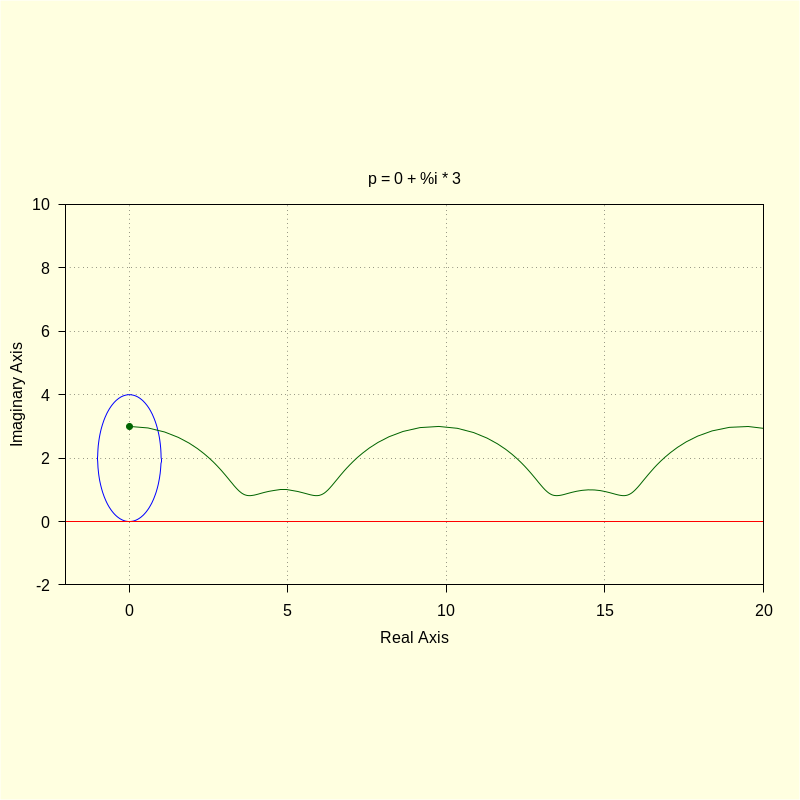
Let's now move p in between the center and the upper focus.
| (%i45) |
a
:
2
$
b
:
1
$
p : %i · 3 ; t : 0 $ tinc : 0 . 1 $ e : 1 − a ^ 2 / b ^ 2 $ for i : 1 thru 400 step 1 do ( u : newton ( b · elliptic_e ( uu , e ) − t , uu , t , 1e-10 ) , roul : fx ( t ) − ( ro ( u , a , b ) − p ) · dfx ( t ) / ( dro ( u , a , b ) · dudt ( u , a , b ) ) , M [ i , 1 ] : float ( realpart ( roul ) ) , M [ i , 2 ] : float ( imagpart ( roul ) ) , t : t + tinc ) $ |
\[\operatorname{(p) }3 i\]
| (%i47) |
kill
(
t
,
u
)
$
wxdraw2d ( xrange = [ − 2 , 20 ] , yrange = [ − 2 , 10 ] , color = blue , parametric ( realpart ( ro ( t , a , b ) ) , imagpart ( ro ( t , a , b ) ) , t , 0 , 2 · %pi ) , color = red , parametric ( realpart ( fx ( t ) ) , imagpart ( fx ( t ) ) , t , − 2 , 20 ) , color = darkgreen , point_size = 1 , point_type = 7 , points ( [ [ realpart ( p ) , imagpart ( p ) ] ] ) , point_type = 0 , points_joined = true , points ( M ) , title = "p = 0 + %i * 3" ) $ |
\[\operatorname{ }\]
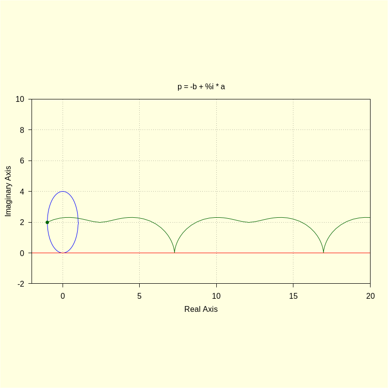
| (%i54) |
a
:
2
$
b
:
1
$
p : − b + %i · a ; t : 0 $ tinc : 0 . 1 $ e : 1 − a ^ 2 / b ^ 2 $ for i : 1 thru 400 step 1 do ( u : newton ( b · elliptic_e ( uu , e ) − t , uu , t , 1e-10 ) , roul : fx ( t ) − ( ro ( u , a , b ) − p ) · dfx ( t ) / ( dro ( u , a , b ) · dudt ( u , a , b ) ) , M [ i , 1 ] : float ( realpart ( roul ) ) , M [ i , 2 ] : float ( imagpart ( roul ) ) , t : t + tinc ) $ |
\[\operatorname{(p) }2 i-1\]
| (%i56) |
kill
(
t
,
u
)
$
wxdraw2d ( xrange = [ − 2 , 20 ] , yrange = [ − 2 , 10 ] , color = blue , parametric ( realpart ( ro ( t , a , b ) ) , imagpart ( ro ( t , a , b ) ) , t , 0 , 2 · %pi ) , color = red , parametric ( realpart ( fx ( t ) ) , imagpart ( fx ( t ) ) , t , − 2 , 20 ) , color = darkgreen , point_size = 1 , point_type = 7 , points ( [ [ realpart ( p ) , imagpart ( p ) ] ] ) , point_type = 0 , points_joined = true , points ( M ) , title = "p = -b + %i * a" ) $ |
\[\operatorname{ }\]
5) Final Comments
The next examples show even more complex (mathematically if not visually) roulettes that are handled using this same method.
Created with
wxMaxima.
Modified and embedded by L.A.P.
We first define the fixed curve (using the parameter t), its derivative, and its arc length. The fixed curve is the real axis (x-axis).