The Web Site of L.A.P.

Roulette Curves with GNU/Linux

1) A Very Complex Roulette: Ellipse Rolling on Limacon

We now attempt a very complex roulette using the method developed previously. This attempt is actually a test of the robustness of the method as it is applied to arbitrary curves. Again, the reader should be familiar with the method for roulette generation that is presented in the introduction.

As usual, we begin with an initialization of Maxima/wxMaxima:

(%i2)

kill ( all ) $ load ( draw ) $ load ( newton1 ) $

(%i3)

set_draw_defaults ( xrange = [ − 2 , 6 ] , yrange = [ − 3 , 3 ] , proportional_axes = xy , grid = true , nticks = 200 , background_color = light_yellow ,
line_type = solid , line_width = 1 ,
   point_type = 0 , point_size = 1 ,
   points_joined = true ,
   xaxis = false , yaxis = false ,
   xlabel = "Real Axis" , ylabel = "Imaginary Axis"
) $

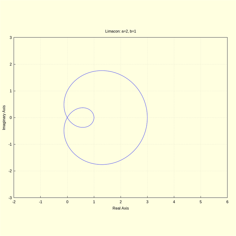
1.1 Define the Fixed Curve as a General Limacon

(%i4)

fx ( t , a , b ) : = ( b + a · cos ( t ) ) · cos ( t ) + %i · ( b + a · cos ( t ) ) · sin ( t ) ;

\[\operatorname{ }\operatorname{fx}\left( t\operatorname{,}a\operatorname{,}b\right) \operatorname{:=}\left( b+a \cos{(t)}\right) \cos{(t)}+i \left( b+a \cos{(t)}\right) \sin{(t)}\]

The fixed curve is paramaterized with t.

The parameters for a specific limacon are chosen to avoid cusps where the first derivative would be undefined. Also, a too sharp curvature would cause convergence problems for the numerical routines that necessarily must be used.

(%i8)

a : 2 $ b : 1 $
wxdraw2d ( nticks = 200 , parametric ( realpart ( fx ( t , a , b ) ) , imagpart ( fx ( t , a , b ) ) , t , 0 , 2 · %pi ) ) $
kill ( a , b ) $

\[\operatorname{ }\]

The following image shows the limacon curve that will be used as the fixed curve:

We now derive the first derivative, dfx(), and the arc length function, sfx().

(%i9)

define ( dfx ( t , a , b ) , trigsimp ( diff ( fx ( t , a , b ) , t ) ) ) ;

\[\operatorname{ }\operatorname{dfx}\left( t\operatorname{,}a\operatorname{,}b\right) \operatorname{:=}\left( -2 a \cos{(t)}-b\right) \sin{(t)}+2 i a {{\cos{(t)}}^{2}}+i b \cos{(t)}-i a\]

(%i10)

integrate ( trigsimp ( cabs ( dfx ( t , a , b ) ) ) , t ) ;

\[\operatorname{ }\int {\left. \sqrt{2 a b \cos{(t)}+{{b}^{2}}+{{a}^{2}}}dt\right.}\]

Again, elliptic integrals are involved in the arc length. Mathworld gives:
2 * (a + b) * elliptic_e(t/2, (4 a b)/(a + b)^2) + constant

(%i11)

sfx ( t , a , b ) : = 2 · ( a + b ) · elliptic_e ( t / 2 , ( 4 · a · b ) / ( a + b ) ^ 2 ) ;

\[\operatorname{ }\operatorname{sfx}\left( t\operatorname{,}a\operatorname{,}b\right) \operatorname{:=}2 \left( a+b\right) \operatorname{elliptic\_ e}\left( \frac{t}{2}\operatorname{,}\frac{4 a b}{{{\left( a+b\right) }^{2}}}\right) \]

1.2 Define the Rolling Curve as a General Ellipse

The rolling curve is an ellipse in standard form with parameters u, ar, br, with ar>br and center at (a+b)+ar.
The ellipse rolls counterclockwise, starting at u - pi.

The first derivative and arc length are now derived.

(%i13)

define ( ro ( u , ar , br , a , b ) , trigsimp ( ar · cos ( − u − %pi ) + %i · br · sin ( − u − %pi ) + ( a + b ) + ar ) ) ;
define ( dro ( u , ar , br ) , diff ( ro ( u , ar , br , a , b ) , u ) ) ;

\[\operatorname{ }\operatorname{ro}\left( u\operatorname{,}\ensuremath{\mathrm{ar}}\operatorname{,}\ensuremath{\mathrm{br}}\operatorname{,}a\operatorname{,}b\right) \operatorname{:=}i \ensuremath{\mathrm{br}} \sin{(u)}-\ensuremath{\mathrm{ar}} \cos{(u)}+b+\ensuremath{\mathrm{ar}}+a\]

\[\operatorname{ }\operatorname{dro}\left( u\operatorname{,}\ensuremath{\mathrm{ar}}\operatorname{,}\ensuremath{\mathrm{br}}\right) \operatorname{:=}\ensuremath{\mathrm{ar}} \sin{(u)}+i \ensuremath{\mathrm{br}} \cos{(u)}\]

(%i14)

' integrate ( cabs ( dro ( u , ar , br ) ) , u ) ;

\[\operatorname{ }\int {\left. \sqrt{{{\ensuremath{\mathrm{ar}}}^{2}} {{\sin{(u)}}^{2}}+{{\ensuremath{\mathrm{br}}}^{2}} {{\cos{(u)}}^{2}}}du\right.}\]

Mathworld gives:
sro(u,ar,br):= br*elliptic_e(u, 1-ar^2/br^2)

(%i15)

sro ( u , ar , br ) : = br · elliptic_e ( u , 1 − ar ^ 2 / br ^ 2 ) ;

\[\operatorname{ }\operatorname{sro}\left( u\operatorname{,}\ensuremath{\mathrm{ar}}\operatorname{,}\ensuremath{\mathrm{br}}\right) \operatorname{:=}\ensuremath{\mathrm{br}} \operatorname{elliptic\_ e}\left( u\operatorname{,}1-\frac{{{\ensuremath{\mathrm{ar}}}^{2}}}{{{\ensuremath{\mathrm{br}}}^{2}}}\right) \]

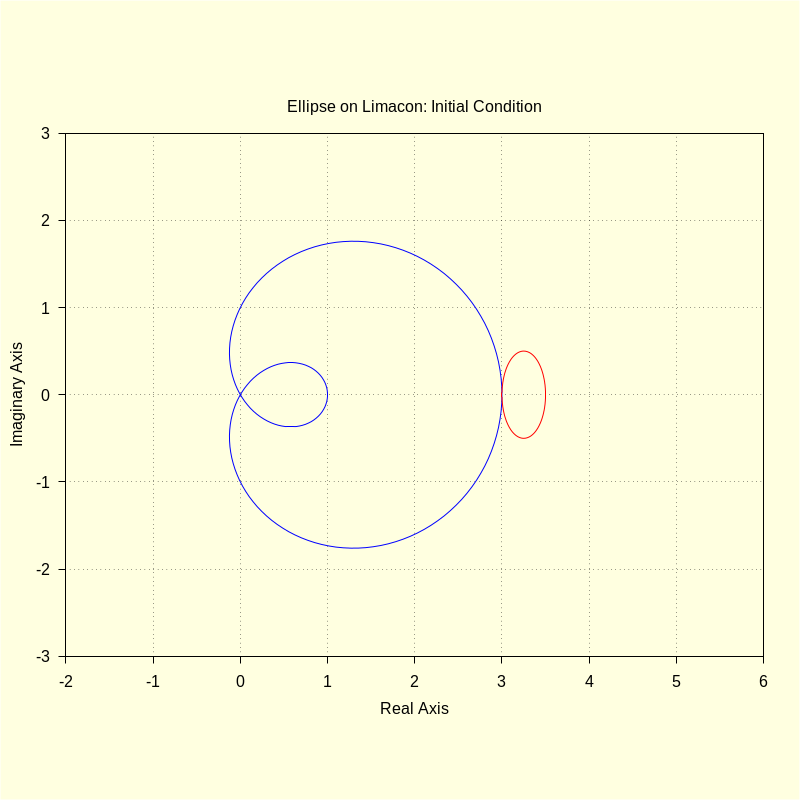
1.3 Plot Initial Condition

(%i21)

a : 2 $ b : 1 $
ar : 1 / 4 $ br : 1 / 2 $
wxdraw2d ( color = blue , parametric ( realpart ( fx ( t , a , b ) ) , imagpart ( fx ( t , a , b ) ) , t , 0 , 2 · %pi ) ,
color = red , parametric ( realpart ( ro ( u , ar , br , a , b ) ) , imagpart ( ro ( u , ar , br , a , b ) ) , u , 0 , 2 · %pi ) ,
title = "Ellipse on Limacon: Initial Condition" ) $
kill ( a , b , ar , br ) $

\[\operatorname{ }\]

1.4 Test the Derived Equations for Correctness

(%i22)

kill ( t , u , ar , br , a , b ) $

We determine, numerically, u(t) for an arbitrary value of t.

(%i28)

t : 100 . 0 ;
a : 2 $ b : 1 $ ar : 1 / 4 $ br : 1 / 2 $
ut : newton ( sro ( u , ar , br ) − sfx ( t , a , b ) , u , t , 1e-10 ) ;

\[\operatorname{(t) }100.0\]

\[\operatorname{(ut) }550.4730334731746\]

Given the above values, do the arc lengths equal?

(%i30)

sfx ( t , a , b ) ;
sro ( ut , ar , br ) ;

\[\operatorname{ }212.2619508547393\]

OK. They are equal. Now we find du/dt, the factor that will allow us to re-define the rolling curve derivative at each plotting iteration. (Again, watch the Maxima syntax. There is a lot happening in this single line.)

(%i32)

kill ( t , u , a , b , ar , br ) $
depends ( u , t ) $

(%i33)

define ( dudt ( t , u , a , b , ar , br ) , radcan ( trigsimp ( rhs ( solve ( factor ( cabs ( diff ( ro ( u , ar , br , a , b ) , t ) ) ) = cabs ( dfx ( t , a , b ) ) , diff ( u , t ) ) [ 1 ] ) ) ) ) ;

\[\operatorname{ }\operatorname{dudt}\left( t\operatorname{,}u\operatorname{,}a\operatorname{,}b\operatorname{,}\ensuremath{\mathrm{ar}}\operatorname{,}\ensuremath{\mathrm{br}}\right) \operatorname{:=}\frac{\sqrt{2 a b \cos{(t)}+{{b}^{2}}+{{a}^{2}}}}{\sqrt{{{\ensuremath{\mathrm{ar}}}^{2}} {{\sin{(u)}}^{2}}+{{\ensuremath{\mathrm{br}}}^{2}} {{\cos{(u)}}^{2}}}}\]

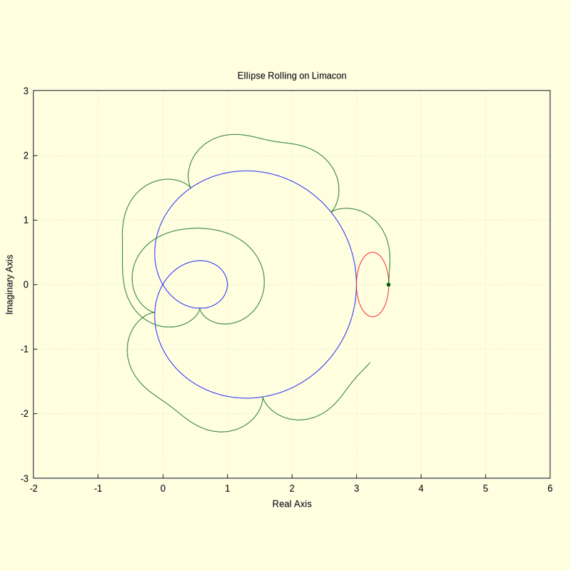
1.5 Plot the Roulette

(%i35)

kill ( t , u , a , b , ar , br , ut , M ) $
M : zeromatrix ( 600 , 2 ) $

(%i43)

a : 2 $ b : 1 $ ar : 1 / 4 $ br : 1 / 2 $
/* p:(a+b)+ar+sqrt(ar^2-br^2)$ */
p : ( a + b ) + 2 · ar $
t : 0 . 0 $ tinc : 0 . 01 $
for i : 1 thru 600 step 1 do (
u : newton ( sro ( ut , ar , br ) − sfx ( t , a , b ) , ut , t , 1e-10 ) ,
roul : fx ( t , a , b ) − ( ro ( u , ar , br , a , b ) − p ) · dfx ( t , a , b ) / ( dro ( u , ar , br ) · dudt ( t , u , a , b , ar , br ) ) ,
M [ i , 1 ] : float ( realpart ( roul ) ) ,
M [ i , 2 ] : float ( imagpart ( roul ) ) ,
t : t + tinc
) $

(%i45)

kill ( u , t ) $
wxdraw2d ( color = blue , parametric ( realpart ( fx ( t , a , b ) ) , imagpart ( fx ( t , a , b ) ) , t , 0 , 2 · %pi ) ,
color = red , parametric ( realpart ( ro ( u , ar , br , a , b ) ) , imagpart ( ro ( u , ar , br , a , b ) ) , u , 0 , 2 · %pi ) ,
color = darkgreen , point_size = 1 , point_type = 7 , points ( [ [ realpart ( p ) , imagpart ( p ) ] ] ) , point_type = 0 , points ( M )
) $

\[\operatorname{ }\]

2) Conclusion

The method that was developed in previous pages does indeed work for arbitrary cases. Provided we can find some procedure, either analytical or numerical, to determine the arc lengths of the fixed and rolling curves then we can create a plot of the roulette.

Created with wxMaxima.
Modified and embedded by L.A.P.