The Web Site of L.A.P.

Geodesics on a Sphere: An Exploration with Maxima/wxMaxima

The sphere is a comparatively simple surface but its general geodesics, aside from the lines of longitude and the equator, are more complex. Nevertheless, the closed equations of the general sphere geodesic can be derived although we shall not do so here. Our purpose is to utilize the derived equations to explore, using Maxima/wxMaxima, some of the geometric properties of the sphere geodesic curve.

Differential geometry (DG) is a vast subject that cannot be expounded in this simple article. The reader is assumed to have a basic knowledge of DG as this article attempts only to demonstrate the use of Maxima/wxMaxima to eliminate the sheer drudgery of very complex DG computations. Also, graphical plots and narrated videos are given using Geomview/StageTools. These graphics are essential in conveying the underlying DG concepts. After all, geometry, differential or otherwise, has always been primarily visual.

A familiarity with the Maxima syntax is also assumed.

The goal, perhaps, of this article, and my other articles on DG, is to elevate one beyond the tedious mathematical formalism of DG and to provide a more visceral insight.

The actual Maxima/wxMaxima script for this article is located here. Please download to reproduce these results on your own machine.

1 The parametric sphere and intrinsic properties thereof

The first step is to initialize the Maxima/wxMaxima environment:

(%i3)

kill(all)$ load(vect)$ load(draw)$
set_draw_defaults(head_angle=10, head_length=0.02, line_width=2, proportional_axes=xyz, nticks=200, xyplane=0, surface_hide=true, point_size=3, point_type=filled_circle, point_size=1)$

A standard parametric equation for the sphere is now defined and also the first and second partial derivatives. The variable names follow the convention stated in my previous article of the Monkey Saddle.

In this case of the sphere, the parameter $u$ is colatitude (θ), $ [0, π] $, and $v$ is longitude (φ), $ [0, 2π] $.

(%i10)

f: [sin(u)*cos(v), sin(u)*sin(v), cos(u)];
fu:diff(f,u);
fv:diff(f,v);
fuu:diff(fu,u);
fuv:diff(fu,v);
fvu:diff(fv,u);
fvv:diff(fv,v);

\[ \mathbf{f} = \left[ \sin{(u)} \cos{(v)}\mathop{,}\sin{(u)} \sin{(v)}\mathop{,}\cos{(u)}\right] \]

\[ \mathbf{fu} = \left[ \cos{(u)} \cos{(v)}\mathop{,}\cos{(u)} \sin{(v)}\mathop{,}\mathop{-}\sin{(u)}\right] \]

\[ \mathbf{fv} = \left[ \mathop{-}\left( \sin{(u)} \sin{(v)}\right) \mathop{,}\sin{(u)} \cos{(v)}\mathop{,}0\right] \]

\[ \mathbf{fuu} = \left[ \mathop{-}\left( \sin{(u)} \cos{(v)}\right) \mathop{,}\mathop{-}\left( \sin{(u)} \sin{(v)}\right) \mathop{,}\mathop{-}\cos{(u)}\right] \]

\[ \mathbf{fuv} = \left[ \mathop{-}\left( \cos{(u)} \sin{(v)}\right) \mathop{,}\cos{(u)} \cos{(v)}\mathop{,}0\right] \]

\[ \mathbf{fvu} = \left[ \mathop{-}\left( \cos{(u)} \sin{(v)}\right) \mathop{,}\cos{(u)} \cos{(v)}\mathop{,}0\right] \]

\[ \mathbf{fvv} = \left[ \mathop{-}\left( \sin{(u)} \cos{(v)}\right) \mathop{,}\mathop{-}\left( \sin{(u)} \sin{(v)}\right) \mathop{,}0\right] \]

The sphere metric and inverse metric are now determined as these are intrinsic geometric properties and will be needed later:

(%i15)

E:trigsimp(fu.fu)$
F:trigsimp(fu.fv)$
G:trigsimp(fv.fv)$
g:trigsimp(matrix([fu.fu, fu.fv],[fv.fu, fv.fv]));
ginv:trigsimp(invert(g));

\[ \mathbf{g} = \begin{bmatrix}1 & 0\\ 0 & {{\sin{(u)}}^{2}}\end{bmatrix}\]

\[ \mathbf{ginv} = \begin{bmatrix}1 & 0\\ 0 & \frac{1}{{{\sin{(u)}}^{2}}}\end{bmatrix}\]

A check to see if the matrix product gives the unit matrix:

(%i16)

trigsimp(g.ginv);

\[ \begin{bmatrix}1 & 0\\ 0 & 1\end{bmatrix}\]

We now derive the unit surface normal, $ n $, of this spherical surface:

(%i18)

tmp:trigsimp(express(fu~fv))$
n:trigsimp(tmp/sqrt(tmp.tmp));

\[ \mathbf{n} = \left[ \left| \sin{(u)}\right| \cos{(v)}\mathop{,}\left| \sin{(u)}\right| \sin{(v)}\mathop{,}\frac{\cos{(u)} \sin{(u)}}{\left| \sin{(u)}\right| }\right] \]

The Christoffel symbols of the sphere are also determined. These are also intrinsic geometric properties that will be utilized later:

(%i20)

load(ctensor)$
init_ctensor()$

(%i24)

dim:2$ ct_coords:[u,v]$
lg:g$
ug:ginv$

(%i25)

christof(mcs)$

We need to re-express the Christoffel symbols as the Maxima result differs from what is used in standard texts on DG:

(%i34)

Γ111:mcs[1,1,1];
Γ112:mcs[1,2,1];
Γ121:mcs[2,1,1];
Γ122:mcs[2,2,1];
Γ211:mcs[1,1,2];
Γ212:mcs[1,2,2];
Γ221:mcs[2,1,2];
Γ222:mcs[2,2,2];

\[ \Gamma^{1}_{11} = 0\]

\[ \Gamma^{1}_{12} = 0\]

\[ \Gamma^{1}_{21} = 0\]

\[ \Gamma^{1}_{22} = \mathop{-}\left( \cos{(u)} \sin{(u)}\right) \]

\[ \Gamma^{2}_{11} = 0\]

\[ \Gamma^{2}_{12} = \frac{\cos{(u)}}{\sin{(u)}}\]

\[ \Gamma^{2}_{21} = \frac{\cos{(u)}}{\sin{(u)}}\]

\[ \Gamma^{2}_{22} = 0\]

2 The general geodesics of the sphere

The geodesics on the sphere can be derived exactly. The method, which gives the colatitude, $ u $, and longitude, $ v $, in terms of a parameter, $ t $, is described in this linked file: sphere.geodesics.pdf

The parametric equations are as follows:

\[ u = \arccos(\sqrt{(1-m^2)} \cdot \sin(t/R)) \]

\[ v = \arctan(m \cdot \tan(t/R)) + v0 \]

In this example, we let $ m = -1/2 $, $ v0 = 0 $, and $ R = 1 $. The curve is evaluated on the surface by substituting the parametric forms of $ u $ and $ v $ into the surface equation $ \mathbf{f} $.

Also, to simplify the equations a bit, we limit $ t \in [-\pi/2, \pi/2] $ which puts a nice constraint on $ \cos(t) $.

(%i38)

/* We will limit t in our plots to [-π/2, π/2] to simplify the equations */
assume(cos(t)>=0)$
m:-1/2$
c:trigsimp(ev(f, u=acos(sqrt(1-m^2)*sin(t)), v=atan(m*tan(t))));
ct:trigsimp(diff(c,t));

\[ c = \left[ \cos{(t)}\mathop{,}\mathop{-}\left( \frac{\sin{(t)}}{2}\right) \mathop{,}\frac{\sqrt{3} \sin{(t)}}{2}\right] \]

\[ ct = \left[ \mathop{-}\sin{(t)}\mathop{,}\mathop{-}\left( \frac{\cos{(t)}}{2}\right) \mathop{,}\frac{\sqrt{3} \cos{(t)}}{2}\right] \]

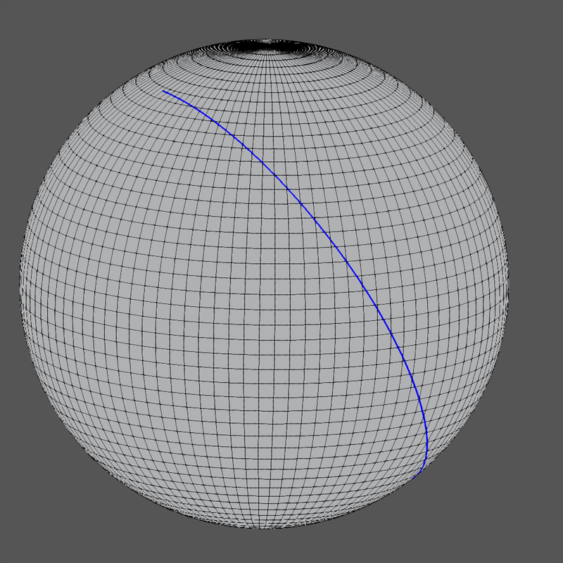
Now comes a plot of the general geodesic, which is shown in blue. Note that our limits on the parameter, $ t $, leads to a "semicircle" which does not encompass the entire surface but that is all that we require for this demonstration. By varying the factors $ m $ and $ v0 $ we can construct a geodesic through any two points on the sphere.

Click Image for Narrated Video

Link for StageTools Script

Check if geodesic is unit speed, i.e. if the curve tangent length is constant and equal to $ 1 $:

(%i40)

trigreduce(trigsimp(sqrt(ct.ct)));

\[ 1 \]

Find the unit normal (determined above as $ \mathbf{n} $) in terms of the geodesic curve parameter $ t $:

(%i41)

nt:trigsimp(ev(n, u=acos(sqrt(1-m^2)*sin(t)), v=atan(m*tan(t))));

\[ \mathbf{nt} = \left[ \cos{(t)}\mathop{,}\mathop{-}\left( \frac{\sin{(t)}}{2}\right) \mathop{,}\frac{\sqrt{3} \sin{(t)}}{2}\right] \]

Check if unit length:

(%i42)

trigsimp(nt.nt);

\[ 1 \]

2.1 The local basis vectors, fu and fv, are now expressed in terms of the geodesic curve parameter t:

(%i44)

fut:trigsimp(ev(fu, u=acos(sqrt(1-m^2)*sin(t)), v=atan(m*tan(t))));
fvt:trigsimp(ev(fv, u=acos(sqrt(1-m^2)*sin(t)), v=atan(m*tan(t))));

\[ \mathbf{fut} = \left[ \frac{\sqrt{3} \cos{(t)} \sin{(t)}}{\sqrt{3 {{\cos{(t)}}^{2}}\mathop{+}1}}\mathop{,}\mathop{-}\left( \frac{\sqrt{3} {{\sin{(t)}}^{2}}}{2 \sqrt{3 {{\cos{(t)}}^{2}}\mathop{+}1}}\right) \mathop{,}\mathop{-}\left( \frac{\sqrt{3 {{\cos{(t)}}^{2}}\mathop{+}1}}{2}\right) \right] \]

\[ \mathbf{fvt} = \left[ \frac{\sin{(t)}}{2}\mathop{,}\cos{(t)}\mathop{,}0\right] \]

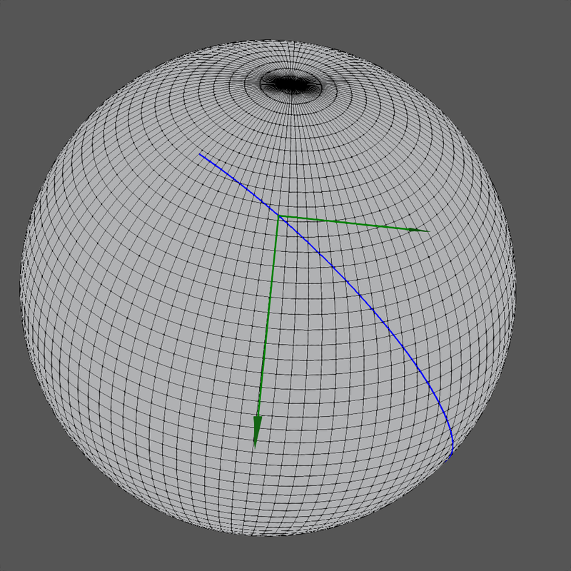
This local basis (shown in green) is now plotted along the geodesic curve. The basis vectors are not normalized and hence will vary in length along the geodesic. Be sure to click the link for a complete and narrated video.

Click Image for Narrated Video

Link for StageTools Script

2.2 Express the tangent to the geodesic curve in terms of the above basis vectors

Find the tangent to geodesic curve $ c $ in terms of un-normalized basis vectors via vector projection,
i.e. $ ct = a \cdot fut + b \cdot fvt $

The derivatives of the coeffients, $ a, b $, are also determined for later use.

(%i49)

a:trigsimp((ct.fut)/(fut.fut));
b:trigsimp((ct.fvt)/(fvt.fvt));
at:trigsimp(diff(a,t));
bt:trigsimp(diff(b,t));

\[ a = \mathop{-}\left( \frac{\sqrt{3} \cos{(t)}}{\sqrt{3 {{\cos{(t)}}^{2}}\mathop{+}1}}\right) \]

\[ b = \mathop{-}\left( \frac{2}{3 {{\cos{(t)}}^{2}}\mathop{+}1}\right) \]

\[ at = \frac{\sqrt{3} \sqrt{3 {{\cos{(t)}}^{2}}\mathop{+}1} \sin{(t)}}{9 {{\cos{(t)}}^{4}}\mathop{+}6 {{\cos{(t)}}^{2}}\mathop{+}1}\]

\[ bt = \mathop{-}\left( \frac{12 \cos{(t)} \sin{(t)}}{9 {{\cos{(t)}}^{4}}\mathop{+}6 {{\cos{(t)}}^{2}}\mathop{+}1}\right) \]

Check if this basis expression equals the geodesic curve tangent (derivative) that was determined above as $ ct $:

(%i51)

trigsimp(trigreduce(trigsimp((a*fut+b*fvt))));
ct;

\[ \left[ \mathop{-}\sin{(t)}\mathop{,}\mathop{-}\left( \frac{\cos{(t)}}{2}\right) \mathop{,}\frac{\sqrt{3} \cos{(t)}}{2}\right] \]

OK. They are equal.

3 The Covariant Derivative of the Geodesic Tangent Vector and General Vectors

3.1 The covariant derivative of the geodesic tangent

We now come to the heart of the exploration. The covariant derivative of the geodesic tangent should be $ 0 $ everywhere because geodesics experience no curvature within the surface (i.e. no geodesic curvature). The geodesic is the generalization of the Euclidian straight line.

First, we need to express the $ u,v $ curve parameters in terms of the geodesic curve parameter $ t $:

(%i53)

ut:trigsimp(diff(acos(sqrt(1-m^2)*sin(t)),t));
vt:trigsimp(diff(atan(m*tan(t)),t));

\[ ut = \mathop{-}\left( \frac{\sqrt{3} \cos{(t)}}{\sqrt{3 {{\cos{(t)}}^{2}}\mathop{+}1}}\right) \]

\[ vt = \mathop{-}\left( \frac{2}{3 {{\cos{(t)}}^{2}}\mathop{+}1}\right) \]

We will now calculate the covariant derivative of the geodesic tangent using the Christoffel symbols:

(%i54)

tmp:(trigsimp((at+Γ111*a*ut + Γ112*a*vt + Γ121*b*ut + Γ122*b*vt)*fut + (bt+Γ211*a*ut + Γ212*a*vt + Γ221*b*ut + Γ222*b*vt)*fvt))$

(%i55)

covd:trigsimp(ev(tmp, u=acos(sqrt(1-m^2)*sin(t)), v=atan(m*tan(t))));

\[ \mathbf{covd} = \left[ 0\mathop{,}0\mathop{,}0\right] \]

Indeed! The covariant derivative of the tangent vector is the zero vector everywhere on the geodesic. Once again, the power of Maxima/wxMaxima to deal with very complex expressions is quite evident.

The covariant derivative can also be determined by subtracting the projection of the directional derivative onto the unit normal from the directional derivative itself. This method, in contrast to the above, is an example of extrinsic geometry, but it serves as a useful check:

(%i56)

dirdiv:trigsimp(diff(ct, t));

\[ \mathbf{dirdiv} = \left[ \mathop{-}\cos{(t)}\mathop{,}\frac{\sin{(t)}}{2}\mathop{,}\mathop{-}\left( \frac{\sqrt{3} \sin{(t)}}{2}\right) \right] \]

(%i57)

covdn:trigsimp(dirdiv-(dirdiv.nt)*nt);

\[ \mathbf{covdn} = \left[ 0\mathop{,}0\mathop{,}0\right] \]

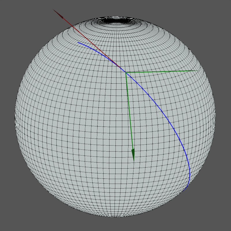
As expected, the result is the same, but the intrinsic method involving Christoffel symbols is preferred.

Now, both the geodesic basis vectors (green) and the geodesic tangent vector (red) are plotted. Be sure to click the link for a complete and narrated video.

Click Image for Narrated Video

Link for StageTools Script

3.2 The covariant derivative of a general vector along the geodesic curve

The geodesic curve tangent is only one of an infinity of vectors in the tangent plane at a given curve point. We now derive the covariant derivative of a general geodesic curve vector: $ \mathbf{V} = a \cdot \mathbf{fut} + b \cdot \mathbf{fvt} $. To make things simple, we use $ a=1, b=1 $ as the vector coefficients. The coefficient derivatives are also determined:

(%i61)

a:1;
b:1;
at:trigsimp(diff(a,t));
bt:trigsimp(diff(b,t));

\[ a = 1\]

\[ b = 1\]

\[ at = 0\]

\[ bt = 0\]

The vector, $ V $, is now expressed:

(%i62)

V:trigsimp(a*fut+b*fvt);

\[ \mathbf{V} = \left[ \frac{\sqrt{3 {{\cos{(t)}}^{2}}\mathop{+}1} \sin{(t)}\mathop{+}2 \sqrt{3} \cos{(t)} \sin{(t)}}{2 \sqrt{3 {{\cos{(t)}}^{2}}\mathop{+}1}}\mathop{,}\frac{2 \cos{(t)} \sqrt{3 {{\cos{(t)}}^{2}}\mathop{+}1}\mathop{-}\sqrt{3} {{\sin{(t)}}^{2}}}{2 \sqrt{3 {{\cos{(t)}}^{2}}\mathop{+}1}}\mathop{,}\mathop{-}\left( \frac{\sqrt{3 {{\cos{(t)}}^{2}}\mathop{+}1}}{2}\right) \right] \]

Using the intrinsic method, with Christoffel symbols, the covariant derivative of vector $ V $ along the geodesic curve is now calculated:

(%i63)

tmp:(trigsimp((at+Γ111*a*ut + Γ112*a*vt + Γ121*b*ut + Γ122*b*vt)*fut + (bt+Γ211*a*ut + Γ212*a*vt + Γ221*b*ut + Γ222*b*vt)*fvt))$

(%i64)

covd:trigsimp(ev(tmp, u=acos(sqrt(1-m^2)*sin(t)), v=atan(m*tan(t))));

\[ \mathbf{covd} = \left[ \frac{\sqrt{3} {{\cos{(t)}}^{2}}\mathop{-}\sqrt{3}}{{{\left( 3 {{\cos{(t)}}^{2}}\mathop{+}1\right) }^{\frac{3}{2}}}}\mathop{,}\mathop{-}\left( \frac{\sqrt{3 {{\cos{(t)}}^{2}}\mathop{+}1} \left( 9 {{\cos{(t)}}^{2}}\mathop{+}3\right) \sin{(t)}\mathop{+}8 \sqrt{3} \cos{(t)} \sin{(t)}}{\sqrt{3 {{\cos{(t)}}^{2}}\mathop{+}1} \left( 12 {{\cos{(t)}}^{2}}\mathop{+}4\right) }\right) \mathop{,}\mathop{-}\left( \frac{\sqrt{3} \sin{(t)}}{4}\right) \right] \]

As expected, the covariant derivative of this general vector is not everywhere equal to $ 0 $.

We now plot the general vector, $ \mathbf{V} $ (in red), and it's covariant derivative (in black) at several points along the geodesic curve along with the basic vectors (in green). Be sure to view the narrated video for a complete description.

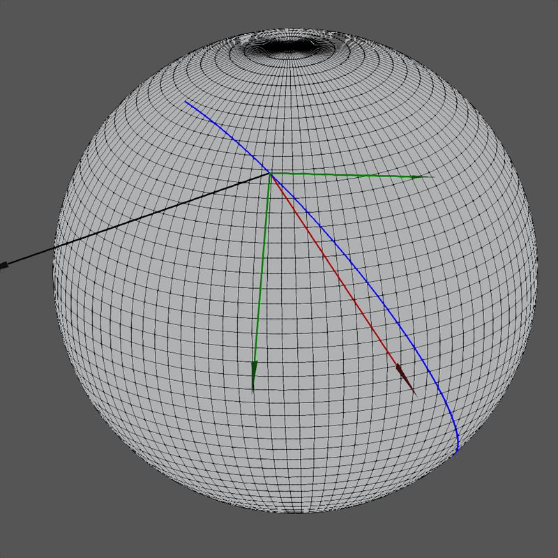
Click Image for Narrated Video

Link for StageTools Script

As a final check, both the general vector, $ \mathbf{V} $, and the covariant derivative should be in the tangent plane, i.e. both should be perpendicular to the unit normal at the same point (their dot products should be $ 0 $).

Is covd perpendicular to the unit normal?

(%i66)

trigsimp(sqrt(covd.nt));

\[ 0\]

Is $ \mathbf{V} $ also in tangent plane (i.e. perpendicular to the normal)?

(%i67)

trigsimp(sqrt(V.nt));

\[ 0\]

4 Final Comments

Again, this article hopefully demonstrates how the use of the Maxima/WxMaxima computer algebra software can eliminate the tediousness of DG and allow a visual insight to be easily developed.

Fortunately, exact geodesic equations are possible for the sphere and this allows geodesic properties to be readily explored. For more complex surfaces, however, this will not necessarily be the case.

Created with wxMaxima
Modified and embedded by L.A.P.