Differential Geometry with GNU/Linux: Monkey Saddle

Differential Geometry with GNU/Linux: The Monkey Saddle Surface with Embedded Parabolic Curve

1 Introductory Spiel

Geometry impresses most people as being a highly visual subject, but opening any textbook on differential geometry (DG) one will find only an endless thicket of mathematical symbols, usually inconsistent from text to text, with only a tiny smattering of visual graphics if any at all. Even actual concrete examples, i.e. practical problems, are rare to find. Mathematical rigor is, beyond doubt, of prime importance but the true beauty, I believe, of DG can only be conveyed through practical examples and above all imagery. The difficulty presumably lies in the extremely tedious and complex nature of problem solving in DG. This is likely why the only practical examples that are given are limited to simple cases like the Euclidian plane (an anti-example?) or the cylinder and sphere.

The rise of computer algebra software (CAS), however, has now made this tedium a thing of the past. Using Maxima CAS, and its graphical front end wxMaxima, both products of FOSS, as I will attempt to show, can allow differential geometry to be explored in a way that reveals its true power and beauty by nearly effortlessly plowing through the complex calculations and graph production.

Because the details of 2D embedded surfaces and curves are best revealed through animation, I have chosen the Geomview software in conjunction with its StageTools module for rapid visualization of the graphics.

This demo is not intended to be a primer of any sort on DG. The subject is far too vast to be covered in a few web pages. I only hope to convey an appreciation for the use of Maxima or other CAS in making DG more intuitive by introducing practical examples and graphics. The reader should already be somewhat versed in the rudiments of DG as I will devote little or no effort in explaining any concepts.

The reader is encouraged to download the actual Maxima workbook and Geomview/Stagetools files for this demo and to execute them on his own machine. Only in this way can the graphics be best appreciated.

Link for wxMaxima Workbook

2 The Monkey Saddle and Curves Thereon

We first initialize the Maxima environment:

(%i1)

kill(all)$

(%i4)

load(vect)$ load(draw)$ load(eigen)$ load(ctensor)$

(%i5)

set_draw_defaults(head_angle=10, head_length=0.03, proportional_axes=xyz, nticks=800, xyplane=0, surface_hide=true, line_width=2, view=[62, 140])$

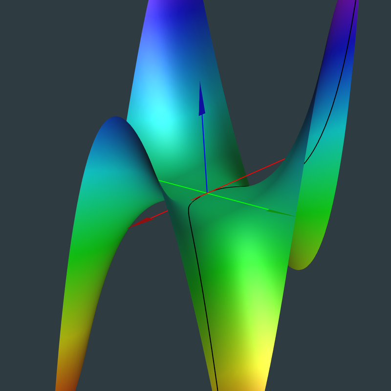
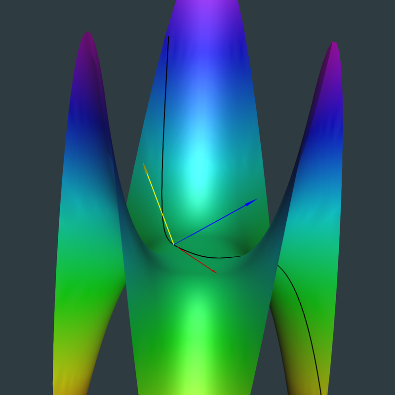
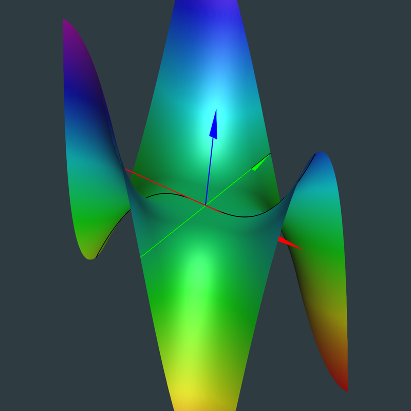
2.1 Define the surface, the monkey saddle

As usual in DG, we consider a mapping from the $ u,v $ plane to the $ x,y,z $ space. Geometrically, the monkey saddle, a relatively complex surface, has the following mapping:

\[ f(u, v) = [x, y, z] = [u, v, u^3-3 u v^2] \]

In these Maxima demos, we will always use $\mathbf f$ as our surface mapping and $\mathbf c$ as our curve function, with derivatives indicated by a following letter:
\[ \frac{\partial \mathbf{f}}{\partial u} \to fu\]
\[ \frac{\mathrm{d}\mathbf{c}}{\mathrm{d}t} \to ct \]

(%i8)

f: [u,v,u^3-3*u*v^2];
fu:diff(f,u);
fv:diff(f,v);

\[ \mathbf{f} = \left[ u\mathop{,}v\mathop{,}{{u}^{3}}\mathop{-}3 u {{v}^{2}}\right] \]

\[ \mathbf{fu} = \left[ 1\mathop{,}0\mathop{,}3 {{u}^{2}}\mathop{-}3 {{v}^{2}}\right] \]

\[ \mathbf{fv} = \left[ 0\mathop{,}1\mathop{,}\mathop{-}\left( 6 u v\right) \right] \]

Check if our surface is regular by taking the cross product of the partial derivatives: \[ \frac{\partial \mathbf{f}}{\partial u} \times \frac{\partial \mathbf{f}}{\partial v} \]

(%i9)

ratsimp(express(fu~fv));

\[ \left[ 3 {{v}^{2}}\mathop{-}3 {{u}^{2}}\mathop{,}6 u v\mathop{,}1\right] \]

This is a regular surface because the cross product is nowhere 0.

2.2 Define a curve on the surface parameterized with t

We now map a parabolic function, $ u = v^2 $, onto the surface. We also compute several derivatives with respect to t as they will be needed later. The first, second, and third derivatives are indicated, respectively, by $ ct, ctt, cttt $:

(%i15)

/* define u,t in terms of t for later use */
tu:t$ tv:t^2$
c:ev(f, u=tu, v=tv);
ct:diff(c,t);
ctt:diff(c,t,2);
cttt:diff(c,t,3);

\[ \mathbf{c} = \left[ t\mathop{,}{{t}^{2}}\mathop{,}{{t}^{3}}\mathop{-}3 {{t}^{5}}\right] \]

\[ \mathbf{ct} = \left[ 1\mathop{,}2 t\mathop{,}3 {{t}^{2}}\mathop{-}15 {{t}^{4}}\right] \]

\[ \mathbf{ctt} = \left[ 0\mathop{,}2\mathop{,}6 t\mathop{-}60 {{t}^{3}}\right] \]

\[ \mathbf{cttt} = \left[ 0\mathop{,}0\mathop{,}6\mathop{-}180 {{t}^{2}}\right] \]

The curve "velocity," or the length of the first derivative, will also be needed later:

(%i16)

vel:ratsimp(sqrt(ct.ct));

\[ \sqrt{225 {{t}^{8}}\mathop{-}90 {{t}^{6}}\mathop{+}9 {{t}^{4}}\mathop{+}4 {{t}^{2}}\mathop{+}1}\]

Now comes a plot of the surface and embedded curve. To better appreciate this surface and curve, a narrated Geomview/StageTools animation is provided. Click on the image or click here (opens in new window).

Click Image for Narrated Video

Link for StageTools Script

2.3 Curvature parameters of the curve on the surface

Before we determine the basic curvature parameters of this curve, we need to find the arc length to establish an arc length parameterization:

(%i19)

integrate(sqrt(ct.ct),t);

\[ \int \sqrt{{{\left( 3 {{t}^{2}}\mathop{-}15 {{t}^{4}}\right) }^{2}}\mathop{+}4 {{t}^{2}}\mathop{+}1}{\, dt}\]

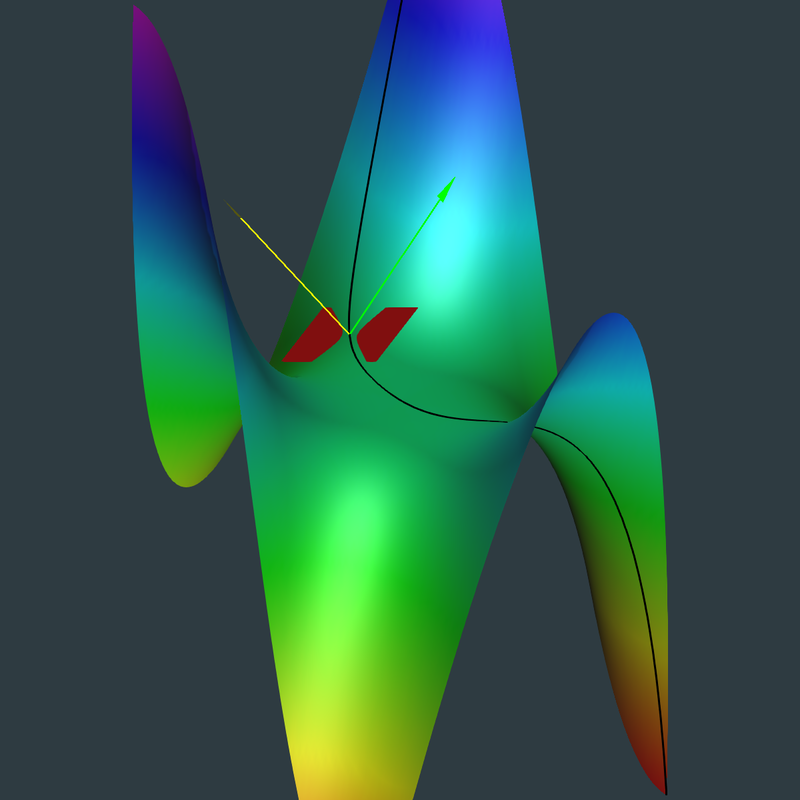
Maxima cannot solve this integral as the solution is not expressible with standard math functions. Even with a solution, function inversion to produce the arc-length parameterization would be problematic. We therefore use the formulas for abitrary speed curves to determine the curvature parameters.

2.3.1 The Darboux moving frame, the unit tangent, T, and unit normal, N, vectors.

Appropriate to a curve embedded within a surface is the Darboux frame which expresses curve properties in terms of surface parameters, namely the geodesic and normal curvatures and the geodesic torsion.

Because the Darboux frame is essentially a rotated version of the Frenet-Serret frame, we need to determine also the Frenet unit vectors.

Unit tangent to curve, $ \mathbf{T} = \frac {c'(t)}{\lvert c'(t) \rvert} $

(%i20)

T:(fullratsimp(ct/sqrt(ct.ct)));

\[ \mathbf{T} = \left[ \frac{1}{\sqrt{225 {{t}^{8}}\mathop{-}90 {{t}^{6}}\mathop{+}9 {{t}^{4}}\mathop{+}4 {{t}^{2}}\mathop{+}1}}\mathop{,}\frac{2 t}{\sqrt{225 {{t}^{8}}\mathop{-}90 {{t}^{6}}\mathop{+}9 {{t}^{4}}\mathop{+}4 {{t}^{2}}\mathop{+}1}}\mathop{,}\mathop{-}\left( \frac{15 {{t}^{4}}\mathop{-}3 {{t}^{2}}}{\sqrt{225 {{t}^{8}}\mathop{-}90 {{t}^{6}}\mathop{+}9 {{t}^{4}}\mathop{+}4 {{t}^{2}}\mathop{+}1}}\right) \right] \]

Check if this is indeed a unit vector:

(%i21)

ratsimp(T.T);

\[ 1\]

The binormal vector: $ \mathbf{B} = \frac{c'(t) \times c''(t)}{\lvert c'(t) \times c''(t) \rvert} $

(%i23)

/* define tmp1 = ct x ctt for later use*/
tmp1:fullratsimp(express(ct~ctt))$
B:fullratsimp(tmp1/sqrt(tmp1.tmp1));

\[ \mathbf{B} = \left[ \mathop{-}\left( \frac{90 {{t}^{4}}\mathop{-}6 {{t}^{2}}}{\sqrt{8100 {{t}^{8}}\mathop{+}2520 {{t}^{6}}\mathop{-}684 {{t}^{4}}\mathop{+}36 {{t}^{2}}\mathop{+}4}}\right) \mathop{,}\frac{60 {{t}^{3}}\mathop{-}6 t}{\sqrt{8100 {{t}^{8}}\mathop{+}2520 {{t}^{6}}\mathop{-}684 {{t}^{4}}\mathop{+}36 {{t}^{2}}\mathop{+}4}}\mathop{,}\frac{2}{\sqrt{8100 {{t}^{8}}\mathop{+}2520 {{t}^{6}}\mathop{-}684 {{t}^{4}}\mathop{+}36 {{t}^{2}}\mathop{+}4}}\right] \]

Check if unit vector:

(%i24)

ratsimp(B.B);

\[ 1\]

Check if T and B are perpendicular. Their cross product should be zero:

(%i25)

ratsimp(B.T);

\[ 0\]

The unit normal: $ \mathbf{N} = \mathbf{B} \times \mathbf{T} $

(%i26)

N:ratsimp(factor(express(B~T)));

\[ \mathbf{N} = \left[ \mathop{-}\left( \frac{450 {{t}^{7}}\mathop{-}135 {{t}^{5}}\mathop{+}9 {{t}^{3}}\mathop{+}2 t}{\sqrt{225 {{t}^{8}}\mathop{-}90 {{t}^{6}}\mathop{+}9 {{t}^{4}}\mathop{+}4 {{t}^{2}}\mathop{+}1} \sqrt{2025 {{t}^{8}}\mathop{+}630 {{t}^{6}}\mathop{-}171 {{t}^{4}}\mathop{+}9 {{t}^{2}}\mathop{+}1}}\right) \mathop{,}\mathop{-}\left( \frac{675 {{t}^{8}}\mathop{-}180 {{t}^{6}}\mathop{+}9 {{t}^{4}}\mathop{-}1}{\sqrt{225 {{t}^{8}}\mathop{-}90 {{t}^{6}}\mathop{+}9 {{t}^{4}}\mathop{+}4 {{t}^{2}}\mathop{+}1} \sqrt{2025 {{t}^{8}}\mathop{+}630 {{t}^{6}}\mathop{-}171 {{t}^{4}}\mathop{+}9 {{t}^{2}}\mathop{+}1}}\right) \mathop{,}\mathop{-}\left( \frac{90 {{t}^{5}}\mathop{+}24 {{t}^{3}}\mathop{-}3 t}{\sqrt{225 {{t}^{8}}\mathop{-}90 {{t}^{6}}\mathop{+}9 {{t}^{4}}\mathop{+}4 {{t}^{2}}\mathop{+}1} \sqrt{2025 {{t}^{8}}\mathop{+}630 {{t}^{6}}\mathop{-}171 {{t}^{4}}\mathop{+}9 {{t}^{2}}\mathop{+}1}}\right) \right] \]

Check if the Frenet frame vectors are mutually perpendicular:

(%i29)

ratsimp(N.N);
ratsimp(N.T);
ratsimp(N.B);

\[ 1\]

\[ 0\]

We now can determine the Darboux Frame vectors: $ \mathbf{T}, \mathbf{nt}, \mathbf{U} $

(%i34)

/* the unit surface normal, $ n $ and its expression, $ nt $, along the curve */
n:express(fu~fv)$
n:fullratsimp(n/sqrt(n.n));
nt:ev(n, u=tu, v=tv);
/* check */
ratsimp(n.n);
ratsimp(nt.nt);

\[ \mathbf{n} = \left[ \frac{3 {{v}^{2}}\mathop{-}3 {{u}^{2}}}{\sqrt{9 {{v}^{4}}\mathop{+}18 {{u}^{2}} {{v}^{2}}\mathop{+}9 {{u}^{4}}\mathop{+}1}}\mathop{,}\frac{6 u v}{\sqrt{9 {{v}^{4}}\mathop{+}18 {{u}^{2}} {{v}^{2}}\mathop{+}9 {{u}^{4}}\mathop{+}1}}\mathop{,}\frac{1}{\sqrt{9 {{v}^{4}}\mathop{+}18 {{u}^{2}} {{v}^{2}}\mathop{+}9 {{u}^{4}}\mathop{+}1}}\right] \]

\[ \mathbf{nt} = \left[ \frac{3 {{t}^{4}}\mathop{-}3 {{t}^{2}}}{\sqrt{9 {{t}^{8}}\mathop{+}18 {{t}^{6}}\mathop{+}9 {{t}^{4}}\mathop{+}1}}\mathop{,}\frac{6 {{t}^{3}}}{\sqrt{9 {{t}^{8}}\mathop{+}18 {{t}^{6}}\mathop{+}9 {{t}^{4}}\mathop{+}1}}\mathop{,}\frac{1}{\sqrt{9 {{t}^{8}}\mathop{+}18 {{t}^{6}}\mathop{+}9 {{t}^{4}}\mathop{+}1}}\right] \]

\[ 1 \]

(%i36)

U:ratsimp(factor(express(nt~T)));
ratsimp(U.U);

\[ \mathbf{U} = \left[ \mathop{-}\left( \frac{90 {{t}^{7}}\mathop{-}18 {{t}^{5}}\mathop{+}2 t}{\sqrt{9 {{t}^{8}}\mathop{+}18 {{t}^{6}}\mathop{+}9 {{t}^{4}}\mathop{+}1} \sqrt{225 {{t}^{8}}\mathop{-}90 {{t}^{6}}\mathop{+}9 {{t}^{4}}\mathop{+}4 {{t}^{2}}\mathop{+}1}}\right) \mathop{,}\frac{45 {{t}^{8}}\mathop{-}54 {{t}^{6}}\mathop{+}9 {{t}^{4}}\mathop{+}1}{\sqrt{9 {{t}^{8}}\mathop{+}18 {{t}^{6}}\mathop{+}9 {{t}^{4}}\mathop{+}1} \sqrt{225 {{t}^{8}}\mathop{-}90 {{t}^{6}}\mathop{+}9 {{t}^{4}}\mathop{+}4 {{t}^{2}}\mathop{+}1}}\mathop{,}\frac{6 {{t}^{5}}\mathop{-}12 {{t}^{3}}}{\sqrt{9 {{t}^{8}}\mathop{+}18 {{t}^{6}}\mathop{+}9 {{t}^{4}}\mathop{+}1} \sqrt{225 {{t}^{8}}\mathop{-}90 {{t}^{6}}\mathop{+}9 {{t}^{4}}\mathop{+}4 {{t}^{2}}\mathop{+}1}}\right] \]

\[ 1 \]

(%i38)

/* $ cos(\theta) $, with $ \theta $ being the rotation angle, using two methods */
radcan(N.U);
radcan(B.nt);

\[ \cos(\theta) = \mathop{-}\left( \frac{135 {{t}^{8}}\mathop{-}324 {{t}^{6}}\mathop{+}27 {{t}^{4}}\mathop{-}1}{\sqrt{9 {{t}^{8}}\mathop{+}18 {{t}^{6}}\mathop{+}9 {{t}^{4}}\mathop{+}1} \sqrt{2025 {{t}^{8}}\mathop{+}630 {{t}^{6}}\mathop{-}171 {{t}^{4}}\mathop{+}9 {{t}^{2}}\mathop{+}1}}\right) \]

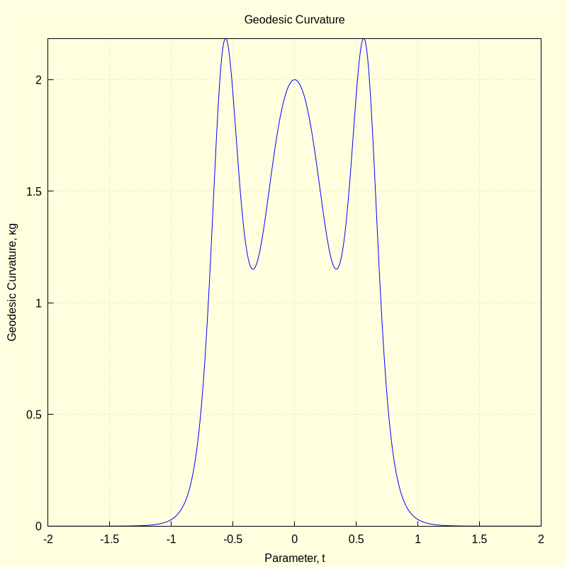
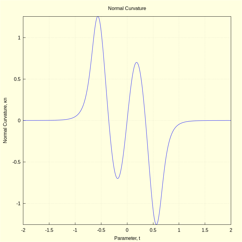
2.3.2 Curvature, $ \kappa $, and the geodesic, $ \kappa g $, and normal, $ \kappa n $, curvatures

$ \kappa = \frac {\lvert c'(t) \times c''(t) \rvert}{\lvert c'(t) \rvert} $

(%i39)

κ:(factor(sqrt(tmp1.tmp1))/(vel^3));

\[ \kappa = \frac{2 \sqrt{2025 {{t}^{8}}\mathop{+}630 {{t}^{6}}\mathop{-}171 {{t}^{4}}\mathop{+}9 {{t}^{2}}\mathop{+}1}}{{{\left( 225 {{t}^{8}}\mathop{-}90 {{t}^{6}}\mathop{+}9 {{t}^{4}}\mathop{+}4 {{t}^{2}}\mathop{+}1\right) }^{\frac{3}{2}}}}\]

(%i40)

/* geodesic curvature */
κg:(ratsimp(ct.(radcan(express(ctt~nt)))))/vel^3;

\[ {\kappa}g = \mathop{-}\left( \frac{270 {{t}^{8}}\mathop{-}648 {{t}^{6}}\mathop{+}54 {{t}^{4}}\mathop{-}2}{\sqrt{9 {{t}^{8}}\mathop{+}18 {{t}^{6}}\mathop{+}9 {{t}^{4}}\mathop{+}1} {{\left( 225 {{t}^{8}}\mathop{-}90 {{t}^{6}}\mathop{+}9 {{t}^{4}}\mathop{+}4 {{t}^{2}}\mathop{+}1\right) }^{\frac{3}{2}}}}\right) \]

(%i41)

/* normal curvature */
/* project curvature, $ \kappa \cdot N $, onto the surface normal, $ n $ */
κn:ratsimp((κ*N).nt);

\[ {\kappa}n = \mathop{-}\left( \frac{48 {{t}^{3}}\mathop{-}6 t}{\sqrt{9 {{t}^{8}}\mathop{+}18 {{t}^{6}}\mathop{+}9 {{t}^{4}}\mathop{+}1} \left( 225 {{t}^{8}}\mathop{-}90 {{t}^{6}}\mathop{+}9 {{t}^{4}}\mathop{+}4 {{t}^{2}}\mathop{+}1\right) }\right) \]

A check of the equality: $ \kappa^2 = {\kappa}n^2 + {\kappa}g^2 $

(%i43)

fullratsimp(factor(κ^2));
fullratsimp(κn^2+κg^2);

\[ \frac{8100 {{t}^{8}}\mathop{+}2520 {{t}^{6}}\mathop{-}684 {{t}^{4}}\mathop{+}36 {{t}^{2}}\mathop{+}4}{11390625 {{t}^{24}}\mathop{-}13668750 {{t}^{22}}\mathop{+}6834375 {{t}^{20}}\mathop{-}1215000 {{t}^{18}}\mathop{-}60750 {{t}^{16}}\mathop{+}2430 {{t}^{14}}\mathop{+}28539 {{t}^{12}}\mathop{-}2808 {{t}^{10}}\mathop{-}810 {{t}^{8}}\mathop{+}10 {{t}^{6}}\mathop{+}75 {{t}^{4}}\mathop{+}12 {{t}^{2}}\mathop{+}1}\]

Now comes a plot of both the geodesic and normal curvatures. Note that all of the "curving" occurs in the interval [-1, 1] with both curvatures falling to zero beyond.

The normal curvature expresses the rotation of the Darboux frame about the U vector while the geodesic curvature expresses the rotation about the normal, N, vector.

(%i44)

wxdraw2d(line_width=1, background_color=light_yellow,
   xlabel="Parameter, t", ylabel="Geodesic Curvature, κg", title="Geodesic Curvature",
   proportional_axes=none, grid=true,
   explicit(κg, t, -2, 2))$

(%i45)

wxdraw2d(line_width=1, background_color=light_yellow,
   xlabel="Parameter, t", ylabel="Normal Curvature, κn", title="Normal Curvature",
   proportional_axes=none,
   explicit(κn, t, -2, 2))$

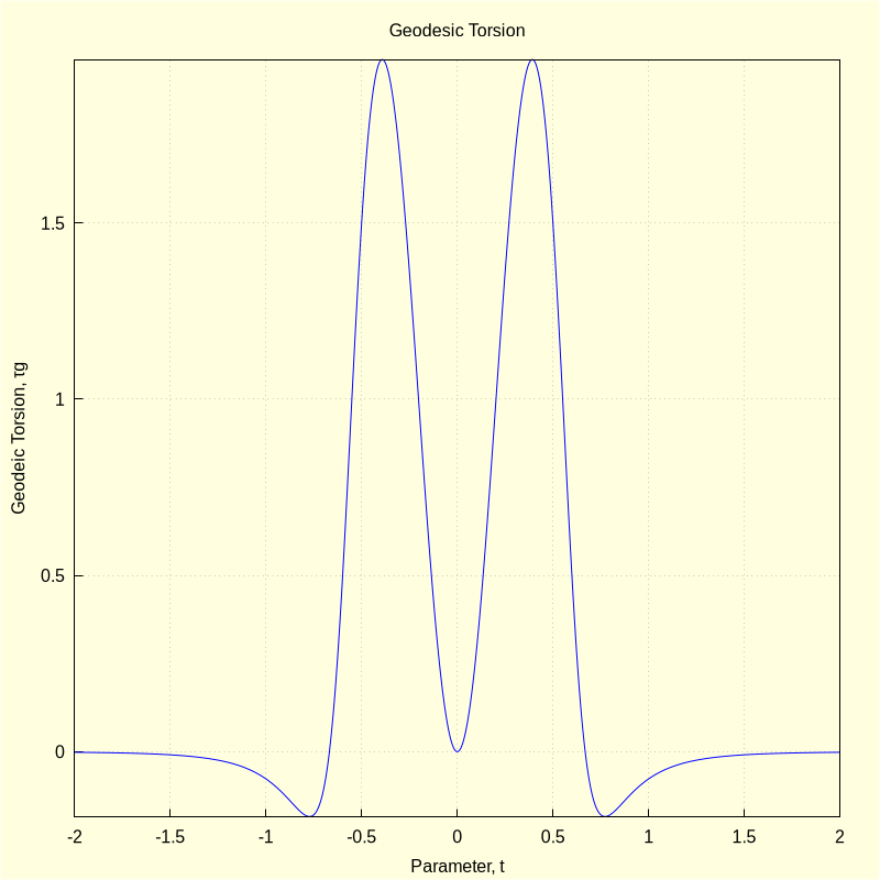
2.3.3 Torsion, $ \tau $, and the geodesic torsion, $ {\tau}g $

Although not strictly necessary for our purposes, we determine the torsion, $ \tau $, of the free curve.

$ \tau = \frac{(c'(t) \times c''(t)) \cdot c'''(t)}{{\lvert c'(t) \times c''(t) \rvert}^2} $

(%i46)

τ:ratsimp(tmp1.cttt)/ratsimp(tmp1.tmp1);

\[ \tau = \frac{12\mathop{-}360 {{t}^{2}}}{8100 {{t}^{8}}\mathop{+}2520 {{t}^{6}}\mathop{-}684 {{t}^{4}}\mathop{+}36 {{t}^{2}}\mathop{+}4}\]

The geodesic torsion, $ {\tau}g $, expresses the rotation of Darboux frame about the tangent, $ \mathbf{T} $, vector.

(%i48)

ntt:ratsimp(factor(diff(nt,t)))$
τg:factor((ratsimp(ct.(radcan(express(ntt~nt)))))/vel^2);

\[ {\tau}g = \mathop{-}\left( \frac{6 {{t}^{2}} \left( 45 {{t}^{8}}\mathop{+}36 {{t}^{6}}\mathop{-}9 {{t}^{4}}\mathop{+}4 {{t}^{2}}\mathop{-}5\right) }{\left( 9 {{t}^{8}}\mathop{+}18 {{t}^{6}}\mathop{+}9 {{t}^{4}}\mathop{+}1\right) \, \left( 225 {{t}^{8}}\mathop{-}90 {{t}^{6}}\mathop{+}9 {{t}^{4}}\mathop{+}4 {{t}^{2}}\mathop{+}1\right) }\right) \]

Now the geodesic torsion is plotted. Again note that most of the "twisting" occurs within the interval [-1, 1].

(%i49)

wxdraw2d(line_width=1, background_color=light_yellow,
   xlabel="Parameter, t", ylabel="Geodeic Torsion, τg", title="Geodesic Torsion",
   proportional_axes=none, grid=true,
   explicit(τg, t, -2, 2))$

A narrated animation, using Geomview/Stagetools, of the moving Darboux frame is now provided. Click on the following still image to open the animation in a new window.

Click Image for Narrated Video

Link for StageTools Script

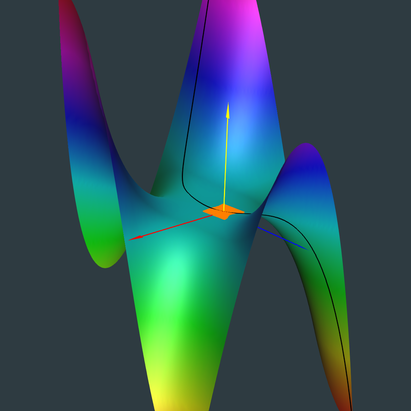
2.4 Curvature Parameters of the Surface (Monkey Saddle)

2.4.1 We now plot the surface unit normal, n, the curve unit normal, N, and the tangent plane, Tp

The general surface tangent plane, $ T_p $, with dummy parameters $u_p$ and $v_p$ specifying the point $ p $:

(%i50)

Tp:[f[1]+up*fu[1]+vp*fv[1], f[2]+up*fu[2]+vp*fv[2], f[3]+up*fu[3]+vp*fv[3]];

\[ T_p = \left[ \ensuremath{\mathrm{u_p}}\mathop{+}u\mathop{,}\ensuremath{\mathrm{v_p}}\mathop{+}v\mathop{,}\mathop{-}\left( 6 u v\, \ensuremath{\mathrm{v_p}}\right) \mathop{-}3 u {{v}^{2}}\mathop{+}\ensuremath{\mathrm{u_p}}\, \left( 3 {{u}^{2}}\mathop{-}3 {{v}^{2}}\right) \mathop{+}{{u}^{3}}\right] \]

(%i51)

/* for plotting along the curve*/
ev(Tp, u=tu, v=tv);

\[ T_p (along \: c) = \left[ \ensuremath{\mathrm{u_p}}\mathop{+}t\mathop{,}\ensuremath{\mathrm{v_p}}\mathop{+}{{t}^{2}}\mathop{,}\mathop{-}\left( 6 {{t}^{3}} \ensuremath{\mathrm{v_p}}\right) \mathop{+}\left( 3 {{t}^{2}}\mathop{-}3 {{t}^{4}}\right) \, \ensuremath{\mathrm{u_p}}\mathop{-}3 {{t}^{5}}\mathop{+}{{t}^{3}}\right] \]

We now plot the tangent plane, and both surface and curve normals, at a specific point, $ u=0.8, v=0.4 $.

Note that the surface normal (yellow), $\mathbf n $, and the curve normal (green), $\mathbf N $, are not the same. (Again,a narrated video using Geomview/StageTools is available by clicking the image.)

Click Image for Narrated Video

Link for StageTools Script

2.4.2 First differential form (metric), $g$

We denote the metric matrix as $g$:

(%i59)

E:fu.fu$
F:fu.fv$
G:fv.fv$
g:matrix([E, F],[F, G]);

\[ g = \begin{bmatrix}{{\left( 3 {{u}^{2}}\mathop{-}3 {{v}^{2}}\right) }^{2}}\mathop{+}1 & \mathop{-}\left( 6 u v\, \left( 3 {{u}^{2}}\mathop{-}3 {{v}^{2}}\right) \right) \\ \mathop{-}\left( 6 u v\, \left( 3 {{u}^{2}}\mathop{-}3 {{v}^{2}}\right) \right) & 36 {{u}^{2}} {{v}^{2}}\mathop{+}1\end{bmatrix}\]

(%i60)

ratsimp(determinant(g));

\[ 9 {{v}^{4}}\mathop{+}18 {{u}^{2}} {{v}^{2}}\mathop{+}9 {{u}^{4}}\mathop{+}1\]

We will also require the metric inverse, $ginv$ later:

(%i61)

ginv:ratsimp(invert(g));

\[ ginv = \begin{bmatrix}\frac{36 {{u}^{2}} {{v}^{2}}\mathop{+}1}{9 {{v}^{4}}\mathop{+}18 {{u}^{2}} {{v}^{2}}\mathop{+}9 {{u}^{4}}\mathop{+}1} & \mathop{-}\left( \frac{18 u {{v}^{3}}\mathop{-}18 {{u}^{3}} v}{9 {{v}^{4}}\mathop{+}18 {{u}^{2}} {{v}^{2}}\mathop{+}9 {{u}^{4}}\mathop{+}1}\right) \\ \mathop{-}\left( \frac{18 u {{v}^{3}}\mathop{-}18 {{u}^{3}} v}{9 {{v}^{4}}\mathop{+}18 {{u}^{2}} {{v}^{2}}\mathop{+}9 {{u}^{4}}\mathop{+}1}\right) & \frac{9 {{v}^{4}}\mathop{-}18 {{u}^{2}} {{v}^{2}}\mathop{+}9 {{u}^{4}}\mathop{+}1}{9 {{v}^{4}}\mathop{+}18 {{u}^{2}} {{v}^{2}}\mathop{+}9 {{u}^{4}}\mathop{+}1}\end{bmatrix}\]

Check. Should give the identity matrix:

(%i62)

ratsimp(g.ginv);

\[ \begin{bmatrix}1 & 0\\ 0 & 1\end{bmatrix}\]

2.4.3 Second differential form, $ b $

Note: The second differential form variables are usually designated $ L, M, N $, but here we use $ NN $ to avoid stepping on the curve unit normal variable, $ \mathbf{N} $.

(%i66)

L:diff(fu,u).n$
M:diff(fu,v).n$
NN:diff(fv,v).n$
b:matrix([L, M], [M, NN]);

\[ b = \begin{bmatrix}\frac{6 u}{\sqrt{9 {{v}^{4}}\mathop{+}18 {{u}^{2}} {{v}^{2}}\mathop{+}9 {{u}^{4}}\mathop{+}1}} & \mathop{-}\left( \frac{6 v}{\sqrt{9 {{v}^{4}}\mathop{+}18 {{u}^{2}} {{v}^{2}}\mathop{+}9 {{u}^{4}}\mathop{+}1}}\right) \\ \mathop{-}\left( \frac{6 v}{\sqrt{9 {{v}^{4}}\mathop{+}18 {{u}^{2}} {{v}^{2}}\mathop{+}9 {{u}^{4}}\mathop{+}1}}\right) & \mathop{-}\left( \frac{6 u}{\sqrt{9 {{v}^{4}}\mathop{+}18 {{u}^{2}} {{v}^{2}}\mathop{+}9 {{u}^{4}}\mathop{+}1}}\right) \end{bmatrix}\]

2.4.4 Shape operator, $ Sp $

The shape operator is defined as the rate of change of the unit normal, i.e. curvature, in a particular direction on the surface. It is an extrinsic curvature.

The coefficients can be found by taking the partial derivatives of the surface normal with respect to the surface parameters:

\[ Sp_u = \frac{\partial \mathbf{n}}{\partial u} \]

\[ Sp_v = \frac{\partial \mathbf{n}}{\partial v} \]

However, the shape operator matrix can also be found as the matrix product of the inverse metric, $ ginv $, with the second fundamental form, $b$.
We use this method as it will be useful immediately below.

(%i67)

Sp:factor(ratsimp(expand(ginv.b)));

\[ Sp = \begin{bmatrix}\frac{6 u\, \left( 18 {{v}^{4}}\mathop{+}18 {{u}^{2}} {{v}^{2}}\mathop{+}1\right) }{{{\left( 9 {{v}^{4}}\mathop{+}18 {{u}^{2}} {{v}^{2}}\mathop{+}9 {{u}^{4}}\mathop{+}1\right) }^{\frac{3}{2}}}} & \mathop{-}\left( \frac{6 v\, \left( 18 {{u}^{2}} {{v}^{2}}\mathop{+}18 {{u}^{4}}\mathop{+}1\right) }{{{\left( 9 {{v}^{4}}\mathop{+}18 {{u}^{2}} {{v}^{2}}\mathop{+}9 {{u}^{4}}\mathop{+}1\right) }^{\frac{3}{2}}}}\right) \\ \mathop{-}\left( \frac{6 v\, \left( 9 {{v}^{4}}\mathop{-}9 {{u}^{4}}\mathop{+}1\right) }{{{\left( 9 {{v}^{4}}\mathop{+}18 {{u}^{2}} {{v}^{2}}\mathop{+}9 {{u}^{4}}\mathop{+}1\right) }^{\frac{3}{2}}}}\right) & \frac{6 u\, \left( 9 {{v}^{4}}\mathop{-}9 {{u}^{4}}\mathop{-}1\right) }{{{\left( 9 {{v}^{4}}\mathop{+}18 {{u}^{2}} {{v}^{2}}\mathop{+}9 {{u}^{4}}\mathop{+}1\right) }^{\frac{3}{2}}}}\end{bmatrix}\]

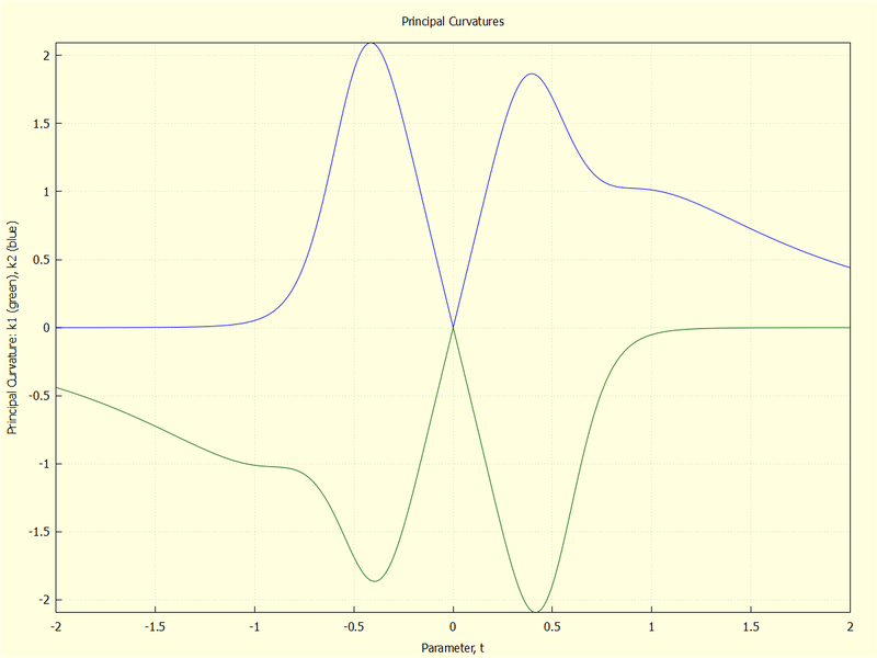
2.4.5 Principal curvatures of the surface

The principal curvature values can be found from the eigenvalues of the shape operator matrix and the principal curvature directions from the eigenvectors. Using Maxima we determine both in one fell swoop:

(%i68)

[spvals,spvects]:eigenvectors(Sp)$

In all their formidable glory, here are the eigenvalues, simplified by Maxima CAS:

(%i70)

pc1:factor(radcan(ratsimp(spvals)))[1][1];
pc2:factor(radcan(ratsimp(spvals)))[1][2];

\[ Sp_{val1} = \mathop{-}\left( \frac{3 \left( \sqrt{{{v}^{2}}\mathop{+}{{u}^{2}}} \sqrt{729 {{u}^{2}} {{v}^{6}}\mathop{+}\left( 243 {{u}^{4}}\mathop{+}36\right) {{v}^{4}}\mathop{+}\left( 72 {{u}^{2}}\mathop{-}405 {{u}^{6}}\right) {{v}^{2}}\mathop{+}81 {{u}^{8}}\mathop{+}36 {{u}^{4}}\mathop{+}4}\mathop{-}27 u {{v}^{4}}\mathop{-}18 {{u}^{3}} {{v}^{2}}\mathop{+}9 {{u}^{5}}\right) }{{{\left( 9 {{v}^{4}}\mathop{+}18 {{u}^{2}} {{v}^{2}}\mathop{+}9 {{u}^{4}}\mathop{+}1\right) }^{\frac{3}{2}}}}\right) \]

\[ Sp_{val2} = \frac{3 \left( \sqrt{{{v}^{2}}\mathop{+}{{u}^{2}}} \sqrt{729 {{u}^{2}} {{v}^{6}}\mathop{+}\left( 243 {{u}^{4}}\mathop{+}36\right) {{v}^{4}}\mathop{+}\left( 72 {{u}^{2}}\mathop{-}405 {{u}^{6}}\right) {{v}^{2}}\mathop{+}81 {{u}^{8}}\mathop{+}36 {{u}^{4}}\mathop{+}4}\mathop{+}27 u {{v}^{4}}\mathop{+}18 {{u}^{3}} {{v}^{2}}\mathop{-}9 {{u}^{5}}\right) }{{{\left( 9 {{v}^{4}}\mathop{+}18 {{u}^{2}} {{v}^{2}}\mathop{+}9 {{u}^{4}}\mathop{+}1\right) }^{\frac{3}{2}}}}\]

Now comes a plot of the principal curvature (PC) values along the embedded curve. Note that the PC values are equal at the origin $ (t=0) $. This point is thus an umbilical point that is identical to a flat plane in terms of curvature.

The PC values are defined anywhere on the surface but here they are plotted only along the embedded curve.

(%i73)

pc1t:ev(pc1, u=tu, v=tv)$
pc2t:ev(pc2, u=tu, v=tv)$
wxdraw2d(line_width=1, background_color=light_yellow,
   xlabel="Parameter, t", ylabel="Principal Curvature: pc1 (green), pc2 (blue)", title="Principal Curvatures",
   proportional_axes=none, grid=true,
   color=dark_green, explicit(pc1t, t, -2, 2),
   color=blue, explicit(pc2t, t, -2, 2)
)$

The eigenvectors contain the components of the principal directions with respect to the tangent basis. That is, the principal directions are obtained by multiplying each basis vector by the appropriate component of the eigenvector. The notation is from the Maxima/wxMaxima output above:

\[ spvects[1][1] \cdot fu + spvects[1][2] \cdot fv\] \[ spvects[2][1] \cdot fu + spvects[2][2] \cdot fv\] The eigenvectors are now shown:

(%i75)

spvec1:radcan(spvects[1][1]);
spvec2:radcan(spvects[2][1]);

\[ Sp_{vec1} = \left[ 1\mathop{,}\frac{\sqrt{{{v}^{2}}\mathop{+}{{u}^{2}}} \sqrt{729 {{u}^{2}} {{v}^{6}}\mathop{+}\left( 243 {{u}^{4}}\mathop{+}36\right) {{v}^{4}}\mathop{+}\left( 72 {{u}^{2}}\mathop{-}405 {{u}^{6}}\right) {{v}^{2}}\mathop{+}81 {{u}^{8}}\mathop{+}36 {{u}^{4}}\mathop{+}4}\mathop{+}9 u {{v}^{4}}\mathop{+}18 {{u}^{3}} {{v}^{2}}\mathop{+}9 {{u}^{5}}\mathop{+}2 u}{36 {{u}^{2}} {{v}^{3}}\mathop{+}\left( 36 {{u}^{4}}\mathop{+}2\right) v}\right] \]

\[ Sp_{vec2} = \left[ 1\mathop{,}\mathop{-}\left( \frac{\sqrt{{{v}^{2}}\mathop{+}{{u}^{2}}} \sqrt{729 {{u}^{2}} {{v}^{6}}\mathop{+}\left( 243 {{u}^{4}}\mathop{+}36\right) {{v}^{4}}\mathop{+}\left( 72 {{u}^{2}}\mathop{-}405 {{u}^{6}}\right) {{v}^{2}}\mathop{+}81 {{u}^{8}}\mathop{+}36 {{u}^{4}}\mathop{+}4}\mathop{-}9 u {{v}^{4}}\mathop{-}18 {{u}^{3}} {{v}^{2}}\mathop{-}9 {{u}^{5}}\mathop{-}2 u}{36 {{u}^{2}} {{v}^{3}}\mathop{+}\left( 36 {{u}^{4}}\mathop{+}2\right) v}\right) \right] \]

Now we check if the principle directions are orthogonal, as they should be.

This is done by first computing the PC vectors according to the formula above and then taking the dot product:

(%i76)

tmp2:(spvec1[1]*fu+spvec1[2]*fv).(spvec2[1]*fu+spvec2[2]*fv);

\[ \left( \frac{6 u v\, \left( \sqrt{{{v}^{2}}\mathop{+}{{u}^{2}}} \sqrt{729 {{u}^{2}} {{v}^{6}}\mathop{+}\left( 243 {{u}^{4}}\mathop{+}36\right) {{v}^{4}}\mathop{+}\left( 72 {{u}^{2}}\mathop{-}405 {{u}^{6}}\right) {{v}^{2}}\mathop{+}81 {{u}^{8}}\mathop{+}36 {{u}^{4}}\mathop{+}4}\mathop{-}9 u {{v}^{4}}\mathop{-}18 {{u}^{3}} {{v}^{2}}\mathop{-}9 {{u}^{5}}\mathop{-}2 u\right) }{36 {{u}^{2}} {{v}^{3}}\mathop{+}\left( 36 {{u}^{4}}\mathop{+}2\right) v}\mathop{-}3 {{v}^{2}}\mathop{+}3 {{u}^{2}}\right) \, \left( \mathop{-}\left( \frac{6 u v\, \left( \sqrt{{{v}^{2}}\mathop{+}{{u}^{2}}} \sqrt{729 {{u}^{2}} {{v}^{6}}\mathop{+}\left( 243 {{u}^{4}}\mathop{+}36\right) {{v}^{4}}\mathop{+}\left( 72 {{u}^{2}}\mathop{-}405 {{u}^{6}}\right) {{v}^{2}}\mathop{+}81 {{u}^{8}}\mathop{+}36 {{u}^{4}}\mathop{+}4}\mathop{+}9 u {{v}^{4}}\mathop{+}18 {{u}^{3}} {{v}^{2}}\mathop{+}9 {{u}^{5}}\mathop{+}2 u\right) }{36 {{u}^{2}} {{v}^{3}}\mathop{+}\left( 36 {{u}^{4}}\mathop{+}2\right) v}\right) \mathop{-}3 {{v}^{2}}\mathop{+}3 {{u}^{2}}\right) \mathop{-}\mathop{(}\left( \sqrt{{{v}^{2}}\mathop{+}{{u}^{2}}} \sqrt{729 {{u}^{2}} {{v}^{6}}\mathop{+}\left( 243 {{u}^{4}}\mathop{+}36\right) {{v}^{4}}\mathop{+}\left( 72 {{u}^{2}}\mathop{-}405 {{u}^{6}}\right) {{v}^{2}}\mathop{+}81 {{u}^{8}}\mathop{+}36 {{u}^{4}}\mathop{+}4}\mathop{-}9 u {{v}^{4}}\mathop{-}18 {{u}^{3}} {{v}^{2}}\mathop{-}9 {{u}^{5}}\mathop{-}2 u\right) \, \left( \sqrt{{{v}^{2}}\mathop{+}{{u}^{2}}} \sqrt{729 {{u}^{2}} {{v}^{6}}\mathop{+}\left( 243 {{u}^{4}}\mathop{+}36\right) {{v}^{4}}\mathop{+}\left( 72 {{u}^{2}}\mathop{-}405 {{u}^{6}}\right) {{v}^{2}}\mathop{+}81 {{u}^{8}}\mathop{+}36 {{u}^{4}}\mathop{+}4}\mathop{+}9 u {{v}^{4}}\mathop{+}18 {{u}^{3}} {{v}^{2}}\mathop{+}9 {{u}^{5}}\mathop{+}2 u\right) \mathop{)}/{{\left( 36 {{u}^{2}} {{v}^{3}}\mathop{+}\left( 36 {{u}^{4}}\mathop{+}2\right) v\right) }^{2}}\mathop{+}1\]

This mess needs to be simplified:

(%i77)

ratsimp(tmp2);

\[ 0\]

They are orthogonal, and, once again, the power of CAS (Maxima) in making a horrendous calculation easy is demonstrated.

Now, we plot the principal curvature vectors at various points along the embedded curve. But since the lengths of the eigenvectors have no particular geometric significance, we need to first normalize them (make them unit vectors).

The resulting expressions are very complex but Maxima/wxMaxima handles them with ease.

(%i79)

tmp3:fullratsimp(ev(spvec1[1]*fu+spvec1[2]*fv, u=tu, v=tv))$
pcv1:fullratsimp(tmp3/fullratsimp(sqrt(tmp3.tmp3)));

\[ \mathbf{pcv1} = \mathop{[} \frac{\sqrt{648 {{u}^{4}} {{v}^{6}}\mathop{+}\left( 1296 {{u}^{6}}\mathop{+}72 {{u}^{2}}\right) {{v}^{4}}\mathop{+}\left( 648 {{u}^{8}}\mathop{+}72 {{u}^{4}}\mathop{+}2\right) {{v}^{2}}}}{\sqrt{26244 {{u}^{4}} {{v}^{10}}\mathop{+}\left( 34992 {{u}^{6}}\mathop{+}2025 {{u}^{2}}\right) {{v}^{8}}\mathop{+}\sqrt{{{v}^{2}}\mathop{+}{{u}^{2}}} \sqrt{729 {{u}^{2}} {{v}^{6}}\mathop{+}\left( 243 {{u}^{4}}\mathop{+}36\right) {{v}^{4}}\mathop{+}\left( 72 {{u}^{2}}\mathop{-}405 {{u}^{6}}\right) {{v}^{2}}\mathop{+}81 {{u}^{8}}\mathop{+}36 {{u}^{4}}\mathop{+}4} \left( 972 {{u}^{3}} {{v}^{6}}\mathop{+}\left( 648 {{u}^{5}}\mathop{+}45 u\right) {{v}^{4}}\mathop{+}\left( 54 {{u}^{3}}\mathop{-}324 {{u}^{7}}\right) {{v}^{2}}\mathop{+}9 {{u}^{5}}\mathop{+}2 u\right) \mathop{+}\left( \mathop{-}\left( 5832 {{u}^{8}}\right) \mathop{+}4860 {{u}^{4}}\mathop{+}36\right) {{v}^{6}}\mathop{+}\left( \mathop{-}\left( 11664 {{u}^{10}}\right) \mathop{+}3726 {{u}^{6}}\mathop{+}252 {{u}^{2}}\right) {{v}^{4}}\mathop{+}\left( 2916 {{u}^{12}}\mathop{+}972 {{u}^{8}}\mathop{+}252 {{u}^{4}}\mathop{+}4\right) {{v}^{2}}\mathop{+}81 {{u}^{10}}\mathop{+}36 {{u}^{6}}\mathop{+}4 {{u}^{2}}}} \mathop{,} \frac{\sqrt{648 {{u}^{4}} {{v}^{6}}\mathop{+}\left( 1296 {{u}^{6}}\mathop{+}72 {{u}^{2}}\right) {{v}^{4}}\mathop{+}\left( 648 {{u}^{8}}\mathop{+}72 {{u}^{4}}\mathop{+}2\right) {{v}^{2}}} \left( \sqrt{{{v}^{2}}\mathop{+}{{u}^{2}}} \sqrt{729 {{u}^{2}} {{v}^{6}}\mathop{+}\left( 243 {{u}^{4}}\mathop{+}36\right) {{v}^{4}}\mathop{+}\left( 72 {{u}^{2}}\mathop{-}405 {{u}^{6}}\right) {{v}^{2}}\mathop{+}81 {{u}^{8}}\mathop{+}36 {{u}^{4}}\mathop{+}4}\mathop{+}9 u {{v}^{4}}\mathop{+}18 {{u}^{3}} {{v}^{2}}\mathop{+}9 {{u}^{5}}\mathop{+}2 u\right) }{\left( 36 {{u}^{2}} {{v}^{3}}\mathop{+}\left( 36 {{u}^{4}}\mathop{+}2\right) v\right) \sqrt{26244 {{u}^{4}} {{v}^{10}}\mathop{+}\left( 34992 {{u}^{6}}\mathop{+}2025 {{u}^{2}}\right) {{v}^{8}}\mathop{+}\sqrt{{{v}^{2}}\mathop{+}{{u}^{2}}} \sqrt{729 {{u}^{2}} {{v}^{6}}\mathop{+}\left( 243 {{u}^{4}}\mathop{+}36\right) {{v}^{4}}\mathop{+}\left( 72 {{u}^{2}}\mathop{-}405 {{u}^{6}}\right) {{v}^{2}}\mathop{+}81 {{u}^{8}}\mathop{+}36 {{u}^{4}}\mathop{+}4} \left( 972 {{u}^{3}} {{v}^{6}}\mathop{+}\left( 648 {{u}^{5}}\mathop{+}45 u\right) {{v}^{4}}\mathop{+}\left( 54 {{u}^{3}}\mathop{-}324 {{u}^{7}}\right) {{v}^{2}}\mathop{+}9 {{u}^{5}}\mathop{+}2 u\right) \mathop{+}\left( \mathop{-}\left( 5832 {{u}^{8}}\right) \mathop{+}4860 {{u}^{4}}\mathop{+}36\right) {{v}^{6}}\mathop{+}\left( \mathop{-}\left( 11664 {{u}^{10}}\right) \mathop{+}3726 {{u}^{6}}\mathop{+}252 {{u}^{2}}\right) {{v}^{4}}\mathop{+}\left( 2916 {{u}^{12}}\mathop{+}972 {{u}^{8}}\mathop{+}252 {{u}^{4}}\mathop{+}4\right) {{v}^{2}}\mathop{+}81 {{u}^{10}}\mathop{+}36 {{u}^{6}}\mathop{+}4 {{u}^{2}}}} \mathop{,} \mathop{-}\left( \frac{\sqrt{648 {{u}^{4}} {{v}^{6}}\mathop{+}\left( 1296 {{u}^{6}}\mathop{+}72 {{u}^{2}}\right) {{v}^{4}}\mathop{+}\left( 648 {{u}^{8}}\mathop{+}72 {{u}^{4}}\mathop{+}2\right) {{v}^{2}}} \left( 3 u \sqrt{{{v}^{2}}\mathop{+}{{u}^{2}}} \sqrt{729 {{u}^{2}} {{v}^{6}}\mathop{+}\left( 243 {{u}^{4}}\mathop{+}36\right) {{v}^{4}}\mathop{+}\left( 72 {{u}^{2}}\mathop{-}405 {{u}^{6}}\right) {{v}^{2}}\mathop{+}81 {{u}^{8}}\mathop{+}36 {{u}^{4}}\mathop{+}4}\mathop{+}81 {{u}^{2}} {{v}^{4}}\mathop{+}\left( 54 {{u}^{4}}\mathop{+}3\right) {{v}^{2}}\mathop{-}27 {{u}^{6}}\mathop{+}3 {{u}^{2}}\right) }{\left( 18 {{u}^{2}} {{v}^{2}}\mathop{+}18 {{u}^{4}}\mathop{+}1\right) \sqrt{26244 {{u}^{4}} {{v}^{10}}\mathop{+}\left( 34992 {{u}^{6}}\mathop{+}2025 {{u}^{2}}\right) {{v}^{8}}\mathop{+}\sqrt{{{v}^{2}}\mathop{+}{{u}^{2}}} \sqrt{729 {{u}^{2}} {{v}^{6}}\mathop{+}\left( 243 {{u}^{4}}\mathop{+}36\right) {{v}^{4}}\mathop{+}\left( 72 {{u}^{2}}\mathop{-}405 {{u}^{6}}\right) {{v}^{2}}\mathop{+}81 {{u}^{8}}\mathop{+}36 {{u}^{4}}\mathop{+}4} \left( 972 {{u}^{3}} {{v}^{6}}\mathop{+}\left( 648 {{u}^{5}}\mathop{+}45 u\right) {{v}^{4}}\mathop{+}\left( 54 {{u}^{3}}\mathop{-}324 {{u}^{7}}\right) {{v}^{2}}\mathop{+}9 {{u}^{5}}\mathop{+}2 u\right) \mathop{+}\left( \mathop{-}\left( 5832 {{u}^{8}}\right) \mathop{+}4860 {{u}^{4}}\mathop{+}36\right) {{v}^{6}}\mathop{+}\left( \mathop{-}\left( 11664 {{u}^{10}}\right) \mathop{+}3726 {{u}^{6}}\mathop{+}252 {{u}^{2}}\right) {{v}^{4}}\mathop{+}\left( 2916 {{u}^{12}}\mathop{+}972 {{u}^{8}}\mathop{+}252 {{u}^{4}}\mathop{+}4\right) {{v}^{2}}\mathop{+}81 {{u}^{10}}\mathop{+}36 {{u}^{6}}\mathop{+}4 {{u}^{2}}}}\right) \mathop{]} \]

(%i81)

tmp3:fullratsimp(ev(spvec2[1]*fu+spvec2[2]*fv, u=tu, v=tv))$
pcv2:fullratsimp(tmp3/fullratsimp(sqrt(tmp3.tmp3)));

\[ \mathbf{pcv2} = \mathop{[} \frac{\sqrt{648 {{u}^{4}} {{v}^{6}}\mathop{+}\left( 1296 {{u}^{6}}\mathop{+}72 {{u}^{2}}\right) {{v}^{4}}\mathop{+}\left( 648 {{u}^{8}}\mathop{+}72 {{u}^{4}}\mathop{+}2\right) {{v}^{2}}}}{\sqrt{26244 {{u}^{4}} {{v}^{10}}\mathop{+}\left( 34992 {{u}^{6}}\mathop{+}2025 {{u}^{2}}\right) {{v}^{8}}\mathop{+}\sqrt{{{v}^{2}}\mathop{+}{{u}^{2}}} \sqrt{729 {{u}^{2}} {{v}^{6}}\mathop{+}\left( 243 {{u}^{4}}\mathop{+}36\right) {{v}^{4}}\mathop{+}\left( 72 {{u}^{2}}\mathop{-}405 {{u}^{6}}\right) {{v}^{2}}\mathop{+}81 {{u}^{8}}\mathop{+}36 {{u}^{4}}\mathop{+}4} \left( \mathop{-}\left( 972 {{u}^{3}} {{v}^{6}}\right) \mathop{+}\left( \mathop{-}\left( 648 {{u}^{5}}\right) \mathop{-}45 u\right) {{v}^{4}}\mathop{+}\left( 324 {{u}^{7}}\mathop{-}54 {{u}^{3}}\right) {{v}^{2}}\mathop{-}9 {{u}^{5}}\mathop{-}2 u\right) \mathop{+}\left( \mathop{-}\left( 5832 {{u}^{8}}\right) \mathop{+}4860 {{u}^{4}}\mathop{+}36\right) {{v}^{6}}\mathop{+}\left( \mathop{-}\left( 11664 {{u}^{10}}\right) \mathop{+}3726 {{u}^{6}}\mathop{+}252 {{u}^{2}}\right) {{v}^{4}}\mathop{+}\left( 2916 {{u}^{12}}\mathop{+}972 {{u}^{8}}\mathop{+}252 {{u}^{4}}\mathop{+}4\right) {{v}^{2}}\mathop{+}81 {{u}^{10}}\mathop{+}36 {{u}^{6}}\mathop{+}4 {{u}^{2}}}} \mathop{,} \mathop{-} \left( \frac{\sqrt{648 {{u}^{4}} {{v}^{6}}\mathop{+}\left( 1296 {{u}^{6}}\mathop{+}72 {{u}^{2}}\right) {{v}^{4}}\mathop{+}\left( 648 {{u}^{8}}\mathop{+}72 {{u}^{4}}\mathop{+}2\right) {{v}^{2}}} \left( \sqrt{{{v}^{2}}\mathop{+}{{u}^{2}}} \sqrt{729 {{u}^{2}} {{v}^{6}}\mathop{+}\left( 243 {{u}^{4}}\mathop{+}36\right) {{v}^{4}}\mathop{+}\left( 72 {{u}^{2}}\mathop{-}405 {{u}^{6}}\right) {{v}^{2}}\mathop{+}81 {{u}^{8}}\mathop{+}36 {{u}^{4}}\mathop{+}4}\mathop{-}9 u {{v}^{4}}\mathop{-}18 {{u}^{3}} {{v}^{2}}\mathop{-}9 {{u}^{5}}\mathop{-}2 u\right) }{\left( 36 {{u}^{2}} {{v}^{3}}\mathop{+}\left( 36 {{u}^{4}}\mathop{+}2\right) v\right) \sqrt{26244 {{u}^{4}} {{v}^{10}}\mathop{+}\left( 34992 {{u}^{6}}\mathop{+}2025 {{u}^{2}}\right) {{v}^{8}}\mathop{+}\sqrt{{{v}^{2}}\mathop{+}{{u}^{2}}} \sqrt{729 {{u}^{2}} {{v}^{6}}\mathop{+}\left( 243 {{u}^{4}}\mathop{+}36\right) {{v}^{4}}\mathop{+}\left( 72 {{u}^{2}}\mathop{-}405 {{u}^{6}}\right) {{v}^{2}}\mathop{+}81 {{u}^{8}}\mathop{+}36 {{u}^{4}}\mathop{+}4} \left( \mathop{-}\left( 972 {{u}^{3}} {{v}^{6}}\right) \mathop{+}\left( \mathop{-}\left( 648 {{u}^{5}}\right) \mathop{-}45 u\right) {{v}^{4}}\mathop{+}\left( 324 {{u}^{7}}\mathop{-}54 {{u}^{3}}\right) {{v}^{2}}\mathop{-}9 {{u}^{5}}\mathop{-}2 u\right) \mathop{+}\left( \mathop{-}\left( 5832 {{u}^{8}}\right) \mathop{+}4860 {{u}^{4}}\mathop{+}36\right) {{v}^{6}}\mathop{+}\left( \mathop{-}\left( 11664 {{u}^{10}}\right) \mathop{+}3726 {{u}^{6}}\mathop{+}252 {{u}^{2}}\right) {{v}^{4}}\mathop{+}\left( 2916 {{u}^{12}}\mathop{+}972 {{u}^{8}}\mathop{+}252 {{u}^{4}}\mathop{+}4\right) {{v}^{2}}\mathop{+}81 {{u}^{10}}\mathop{+}36 {{u}^{6}}\mathop{+}4 {{u}^{2}}}}\right) \mathop{,} \frac{\sqrt{648 {{u}^{4}} {{v}^{6}}\mathop{+}\left( 1296 {{u}^{6}}\mathop{+}72 {{u}^{2}}\right) {{v}^{4}}\mathop{+}\left( 648 {{u}^{8}}\mathop{+}72 {{u}^{4}}\mathop{+}2\right) {{v}^{2}}} \left( 3 u \sqrt{{{v}^{2}}\mathop{+}{{u}^{2}}} \sqrt{729 {{u}^{2}} {{v}^{6}}\mathop{+}\left( 243 {{u}^{4}}\mathop{+}36\right) {{v}^{4}}\mathop{+}\left( 72 {{u}^{2}}\mathop{-}405 {{u}^{6}}\right) {{v}^{2}}\mathop{+}81 {{u}^{8}}\mathop{+}36 {{u}^{4}}\mathop{+}4}\mathop{-}81 {{u}^{2}} {{v}^{4}}\mathop{+}\left( \mathop{-}\left( 54 {{u}^{4}}\right) \mathop{-}3\right) {{v}^{2}}\mathop{+}27 {{u}^{6}}\mathop{-}3 {{u}^{2}}\right) }{\left( 18 {{u}^{2}} {{v}^{2}}\mathop{+}18 {{u}^{4}}\mathop{+}1\right) \sqrt{26244 {{u}^{4}} {{v}^{10}}\mathop{+}\left( 34992 {{u}^{6}}\mathop{+}2025 {{u}^{2}}\right) {{v}^{8}}\mathop{+}\sqrt{{{v}^{2}}\mathop{+}{{u}^{2}}} \sqrt{729 {{u}^{2}} {{v}^{6}}\mathop{+}\left( 243 {{u}^{4}}\mathop{+}36\right) {{v}^{4}}\mathop{+}\left( 72 {{u}^{2}}\mathop{-}405 {{u}^{6}}\right) {{v}^{2}}\mathop{+}81 {{u}^{8}}\mathop{+}36 {{u}^{4}}\mathop{+}4} \left( \mathop{-}\left( 972 {{u}^{3}} {{v}^{6}}\right) \mathop{+}\left( \mathop{-}\left( 648 {{u}^{5}}\right) \mathop{-}45 u\right) {{v}^{4}}\mathop{+}\left( 324 {{u}^{7}}\mathop{-}54 {{u}^{3}}\right) {{v}^{2}}\mathop{-}9 {{u}^{5}}\mathop{-}2 u\right) \mathop{+}\left( \mathop{-}\left( 5832 {{u}^{8}}\right) \mathop{+}4860 {{u}^{4}}\mathop{+}36\right) {{v}^{6}}\mathop{+}\left( \mathop{-}\left( 11664 {{u}^{10}}\right) \mathop{+}3726 {{u}^{6}}\mathop{+}252 {{u}^{2}}\right) {{v}^{4}}\mathop{+}\left( 2916 {{u}^{12}}\mathop{+}972 {{u}^{8}}\mathop{+}252 {{u}^{4}}\mathop{+}4\right) {{v}^{2}}\mathop{+}81 {{u}^{10}}\mathop{+}36 {{u}^{6}}\mathop{+}4 {{u}^{2}}}} \]

Check if they are both unit vectors and also check if they lie within the tangent plane.

(%i85)

fullratsimp(pcv1.pcv1);
fullratsimp(pcv2.pcv2);
fullratsimp(pcv1.n);
fullratsimp(pcv2.n);

\[ 1\]

\[ 0\]

All is good, so now the plot. Here, the PC unit vectors are scaled with the respective PC values.
For a Geomview/StageTools animated graphic click the image (opens in new window).

Click Image for Video

Link for StageTools Script

2.5 The Christoffel symbols

In Maxima, the Christoffel symbols are found using the "ctensor" package:

(%i63)

load ( ctensor ) $

init_ctensor ( ) $

dim : 2 $ ct_coords : [ u , v ] $
lg : g $
ug : ginv $

(%i69)

christof ( mcs ) $

A peculiarity of Maxima is that the indexing of the Christoffel symbols differs from the conventions used in most DG textbooks. We now rectify this by defining new variables.

The pattern is $ \Gamma_{jk}^i = mcs(j, k, i) $

Γ111 : mcs [ 1 , 1 , 1 ] ;
Γ112 : mcs [ 1 , 2 , 1 ] ;
Γ121 : mcs [ 2 , 1 , 1 ] ;
Γ122 : mcs [ 2 , 2 , 1 ] ;
Γ211 : mcs [ 1 , 1 , 2 ] ;
Γ212 : mcs [ 1 , 2 , 2 ] ;
Γ221 : mcs [ 2 , 1 , 2 ] ;
Γ222 : mcs [ 2 , 2 , 2 ] ;

\[ \Gamma^{1}_{11} = \mathop{-}\left( \frac{18 u {{v}^{2}}\mathop{-}18 {{u}^{3}}}{9 {{v}^{4}}\mathop{+}18 {{u}^{2}} {{v}^{2}}\mathop{+}9 {{u}^{4}}\mathop{+}1}\right) \]

\[ \Gamma^{1}_{12} = \frac{18 {{v}^{3}}\mathop{-}18 {{u}^{2}} v}{9 {{v}^{4}}\mathop{+}18 {{u}^{2}} {{v}^{2}}\mathop{+}9 {{u}^{4}}\mathop{+}1}\]

\[ \Gamma^{1}_{21} = \frac{18 {{v}^{3}}\mathop{-}18 {{u}^{2}} v}{9 {{v}^{4}}\mathop{+}18 {{u}^{2}} {{v}^{2}}\mathop{+}9 {{u}^{4}}\mathop{+}1}\]

\[ \Gamma^{1}_{22} = \frac{18 u {{v}^{2}}\mathop{-}18 {{u}^{3}}}{9 {{v}^{4}}\mathop{+}18 {{u}^{2}} {{v}^{2}}\mathop{+}9 {{u}^{4}}\mathop{+}1}\]

\[ \Gamma^{2}_{11} = \mathop{-}\left( \frac{36 {{u}^{2}} v}{9 {{v}^{4}}\mathop{+}18 {{u}^{2}} {{v}^{2}}\mathop{+}9 {{u}^{4}}\mathop{+}1}\right) \]

\[ \Gamma^{2}_{12} = \frac{36 u {{v}^{2}}}{9 {{v}^{4}}\mathop{+}18 {{u}^{2}} {{v}^{2}}\mathop{+}9 {{u}^{4}}\mathop{+}1}\]

\[ \Gamma^{2}_{21} = \frac{36 u {{v}^{2}}}{9 {{v}^{4}}\mathop{+}18 {{u}^{2}} {{v}^{2}}\mathop{+}9 {{u}^{4}}\mathop{+}1}\]

\[ \Gamma^{2}_{22} = \frac{36 {{u}^{2}} v}{9 {{v}^{4}}\mathop{+}18 {{u}^{2}} {{v}^{2}}\mathop{+}9 {{u}^{4}}\mathop{+}1}\]

2.6 Geodesics of the Monkey Saddle Surface

The geodesic curvature of the parabolic curve, $ c $, that is embedded in the Monkey Saddle surface is not everywhere equal to $ 0 $ and hence the curve is not a geodesic. But what are the geodesics?

The trivial geodesics are the initial coordinate curves: $ [0, t, 0], [t,0,t^3] $

ev(f, u=0, v=t);
ev(f, u=t, v=0);

\[ \left[ 0\mathop{,}t\mathop{,}0\right] \]

\[ \left[ t\mathop{,}0\mathop{,}{{t}^{3}}\right] \]

These are now plotted. To gain the best insight just click the image for a video.

Click Image for Video

Link for StageTools Script

For the general geodesic curve, we need to solve the differential equation system:

\[ u''(t) + \Gamma_{11}^1 u'(t)^2 + 2 \Gamma_{12}^1 u'(t) v'(t) + \Gamma_{22}^1 v'(t)^2 = 0 \]
\[ v''(t) + \Gamma_{11}^2 u'(t)^2 + 2 \Gamma_{12}^2 u'(t) v'(t) + \Gamma_{22}^2 v'(t)^2 = 0 \]
In what follows, the variables $u$, $v$ are to be understood as being functions of the parameter $t$, with subscripts indicating derivatives w/r to $t$.

depends(u,t)$
depends(v,t)$

diff(u,t,2) + Γ111*diff(u,t)^2 + 2*Γ112*diff(u,t)*diff(v,t) + Γ122*diff(v,t)^2;
diff(v,t,2) + Γ211*diff(u,t)^2 + 2*Γ212*diff(u,t)*diff(v,t) + Γ222*diff(v,t)^2;

\[ \frac{\left( 18 u {{v}^{2}}\mathop{-}18 {{u}^{3}}\right) {{\left( {v_t}\right) }^{2}}}{9 {{v}^{4}}\mathop{+}18 {{u}^{2}} {{v}^{2}}\mathop{+}9 {{u}^{4}}\mathop{+}1}\mathop{+}\frac{2 \left( {u_t}\right) \, \left( 18 {{v}^{3}}\mathop{-}18 {{u}^{2}} v\right) \, \left( {v_t}\right) }{9 {{v}^{4}}\mathop{+}18 {{u}^{2}} {{v}^{2}}\mathop{+}9 {{u}^{4}}\mathop{+}1}\mathop{-}\frac{{{\left( {u_t}\right) }^{2}} \left( 18 u {{v}^{2}}\mathop{-}18 {{u}^{3}}\right) }{9 {{v}^{4}}\mathop{+}18 {{u}^{2}} {{v}^{2}}\mathop{+}9 {{u}^{4}}\mathop{+}1}\mathop{+}{u_{tt}}\]

\[ {v_{tt}}\mathop{+}\frac{36 {{u}^{2}} v {{\left( {v_t}\right) }^{2}}}{9 {{v}^{4}}\mathop{+}18 {{u}^{2}} {{v}^{2}}\mathop{+}9 {{u}^{4}}\mathop{+}1}\mathop{+}\frac{72 u\, \left( {u_t}\right) {{v}^{2}} \left( {v_t}\right) }{9 {{v}^{4}}\mathop{+}18 {{u}^{2}} {{v}^{2}}\mathop{+}9 {{u}^{4}}\mathop{+}1}\mathop{-}\frac{36 {{u}^{2}} {{\left( {u_t}\right) }^{2}} v}{9 {{v}^{4}}\mathop{+}18 {{u}^{2}} {{v}^{2}}\mathop{+}9 {{u}^{4}}\mathop{+}1}\]

This is a coupled set of second-order, non-linear differential equations that would need to be solved numerically. The numerical solution, although straightforward and within the capability of Maxima/wxMaxima, would only yield an array of points that would provide no mathematical insight. However, we will demonstrate finding the numerical solution to the Monkey Saddle geodesics in another, dedicated, web page.

3 Epilogue

Differential geometry is a most beautiful and exciting area of mathematics, yet these inspiring aspects are usually obscured by the dull tedium of the often complex derivations and computations that are involved. Using a CAS, however, can liberate one from this dull tedium and allow the underlying beauty and excitement to come forth. The free and open source Maxima/wxMaxima package, as (hopefully) adequately demonstrated in this article, is a perfect tool for exploring differential geometry without getting stalled in the dense and tiresome thicket of manual calculation.

Created with wxMaxima.
Modified and embedded by L.A.P.