Most people, from naive children to seasoned adults, will have an undeniable fascination with rotating objects such as gyroscopes and spinning tops. Their motion seems magical and almost paradoxical but they are always a true joy to observe.

However, their utter simplicity belies their near mathematical intractability. It requires very sophisticated mathematics, namely Lagrangian or Hamilitonian mechanics, to fully describe the motion of these "rigid rotors."

The physical theories of rotation began with Leonhard Eurler in 1776 and culminated in the 19th century masterworks of Lagrange and Hamilton. But even these monumental achievements were not enough. In the 1960's, NASA watched as its Explorer I satellite tumbled out of control due to an incomplete understanding of the mechanics of rotating bodies (technical link).

Thus, the rotating top (or gyroscope) is not as simple at it may seem.

In this article I will demonstrate the use of GNU/Linux software tools to simulate the motion of a spinning symmetric top with friction. Most of this material follows the excellent contributions at rotations.berkeley.edu. I have only reworked the simulations using the GNU Scientific Library and have used the POV Ray rendering software, in conjunction with ffmpeg, to create more vivid animations. The Gnuplot plotting software was used to create the accessory graphs. The Berkeley site should be consulted to clarify any details of the derivations.

But as forewarned, the mathematics is formidable. The reader interested in diving deeper should at least have an undergraduate level of math and physics. The animations, however, can be enjoyed with no background at all. Feel free to skip to the videos below.

The mathematics of rotating bodies is complex but we provide a basic outline of our model of the symmetric top with friction. For the adventurous, the exact developmental details are found within the Matlab scripts at rotations.berkeley.edu.

There are two coordinate systems, both Euclidean and orthonormal, to consider:

1) The stationary, or laboratory, frame with basis \( {\bar{E}_1}\operatorname{,}{\bar{E}_2}\operatorname{,}{\bar{E}_3} \).

2) The co-rotating frame with basis \( {\bar{e}_1}\operatorname{,}{\bar{e}_2}\operatorname{,}{\bar{e}_3} \), with \({\bar{e}_3} \) aligning with the symmetric top axial axis.

(Note: following rotations.berkeley.edu, we use numerical indices, 1, 2, 3, for the basis vectors but they correspond to the common x, y, z notation.)

The position of the top center of mass (CM) is described in the lab frame with coordinates \(\left[ {x_1}\operatorname{,}{x_2}\operatorname{,}{x_3}\right] \).

The rotation of the top is parameterized using the 3-1-3 Euler angles, ψ, θ, φ, with φ indicating rotation, θ nutation, and ψ the precession.

The state vector, which describes the evolution of the top motion, is \( \left[
\psi'\operatorname{,}\theta'\operatorname{,}\phi'\operatorname{,}\psi\operatorname{,}\theta\operatorname{,}\phi\operatorname{,}{x_1}'\operatorname{,}{x_2}'\operatorname{,}{x_1}\operatorname{,}{x_2}\right] \), the primed variables denoting the time derivative. This, of course, means that we will track, through our numerical simulation, the coordinates of the top CM and the orientation in space as a function of time.

To derive the equations of motion we use a basic force and moment balance scheme rather than a Lagrangian or Hamiltonian approach.

The two relevant force and moment balance equations are:

\[ \sum \bar F = m \frac {d^2x_1} {dt^2} \; \bar{E}_1 + m \frac {d^2x_2} {dt^2} \; \bar{E}_2 + m \frac {d^2x_3} {dt^2} \; \bar{E}_3 \]

\[ \sum \bar M = \lambda_t \frac {d\omega_1}{dt} \; \bar{e}_1 + \lambda_t \frac {d\omega_2}{dt} \; \bar{e}_2 + \lambda_a \frac {d\omega_3}{dt} \; \bar{e}_3 \]

where \( \sum \bar F \) is the sum of the forces, \( \sum \bar M \) is the sum of the moments, \( \omega_i \) are the angular velocities, and \( \lambda_t \), \( \lambda_a \) are the transverse and axial moments of inertia.

In addition to the gravitational force, the top also experiences a kinetic friction force as its contact point slides along the surface. This friction force is the only other significant force within our model and is described as follows:

\[ \bar{F}_f = -\mu_k N \frac {\bar{v}_p}{\lVert \bar{v}_p \rVert} \]

where \( \mu_k \) is the coefficient of kinetic friction, N is the normal force at the contact point, and \( \bar{v}_p \) is the vector velocity of the contact point. Both N and \( \bar{v}_p \) can be expressed in terms of the state variables (see the Matlab scripts for details).

The laboratory and rotating frames are related using the 3-1-3 Euler angles. The transformation matrix is derived with wxMaxima as follows:

In order to balance the moments, the components of the angular velocity, \( \omega_i \), need to be expressed in terms of the rates of change of the Euler angles. The following derivation, using wxMaxima, provides the angular velocity vector:

We now have expressions for linear and angular momentum, as well as normal and frictional forces, in terms of the state variables. Performing the balance, we ultimately obtain the equation:

\[ M(y, t) * y(t) = f(t, y) \]

where \( M(y, t) \) is the mass matrix and \( y(t) \) is the state vector (shown above).

Even rotations.berkeley.edu does not explicitly state the details of this very complex derivation. One has to examine the actual Matlab scripts to obtain the full procedure.

One can also examine my C program, which uses GSL numerical routines rather than Matlab, to discover the full set of equations, some of which contain thousands of terms.

However, the important aspect of this simulation is not the detailed derivation but rather the general principles involved, which in this case is a straightforward force and moment balance and coordinate transformations using Euler angles. The complexity and tedium can be addressed with computer algebra software (CAS).

The above equation, \( M(y, t) * y(t) = f(t, y) \), is a system of first order differential equations. These are solved numerically using the ODE solvers of the GNU Scientific Library, in particular the Explicit embedded Runge-Kutta Prince-Dormand (8, 9).

As a final step, the equation is numerically inverted at each time increment, using the GSL BLAS routines, to provide \( y(t) = \left[
\psi'\operatorname{,}\theta'\operatorname{,}\phi'\operatorname{,}\psi\operatorname{,}\theta\operatorname{,}\phi\operatorname{,}{x_1}'\operatorname{,}{x_2}'\operatorname{,}{x_1}\operatorname{,}{x_2}
\right] \), which is the state vector for our model system.

From the values of the state variables, we then calculate the \( x_3 \) coordinate of the CM, the co-rotating basis vectors \( {\bar{e}_1}\operatorname{,}{\bar{e}_2}\operatorname{,}{\bar{e}_3} \), and the components of the angular momentum with respect to the lab (stationary) frame.

The complete, and tedious, details are found in my C program.

These values, which are output to a CSV file, are then used as data for both plotting with gnuplot and POV Ray animations.

POV Ray is a ray-tracing program and was chosen instead of a math plotting package because the resulting graphics can be, if done properly (and I hope that I have done it properly), much more vivid and stunning.

One must keep in mind, however, that POV Ray was not designed for mathematical plotting and further munging of the data has to be done to make it all work. For one thing, POV Ray uses a left handed coordinate system that is transformed with respect to the Euclidean coordinates of our model configutation space.

Basically, the co-rotating basis vectors, \( {\bar{e}_1}\operatorname{,}{\bar{e}_2}\operatorname{,}{\bar{e}_3} \), which are calculated from the Euler angles at each time step, and which form an orthonormal set, are used in the POV Ray transform function Shear_Trans(A, B, C). Because the POV Ray coordinates <x, y, z> are related to Euclidean coordintes [x, y, z] by the relation <x, y, z> = [y, z, -x], the vectors A, B, C are defined as follows:

A = <e2y, e2z, -e2x>
B = <e3y, e3z, -e3x>
C = <e1y, e1z, -e1x>

where e1x is the x component of the \( \bar{e}_1 \) vector, etc.

Using these vectors in Shear_Trans(A, B, C) produces a rotation that is equivalent to using the 3-1-3 Euler angles in Euclidean space.

This rotation is then followed by a POV Ray translation to properly locate the contact point.

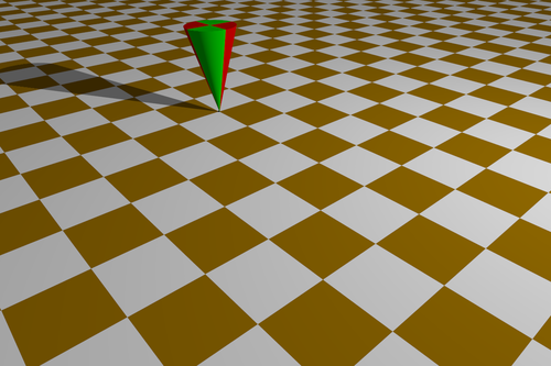
On the POV Ray "checkerboard" one square length equals 20 centimeters. The x-axis runs southwest (positive) to northeast (negative). The y-axis runs northwest (negative) to southeast (positive).

For those interested, the POV Ray file used to render a single step of the animation is here.

Using the GSL C program (top-w-friction.c) a simulation was produced using the following initial and other parameters:

./top-w-friction mass g radius lamdat lamda l3 muk psi' theta' phi' psi phi x1' x2' x1 x2 t0 tmax tinc > top.csv

Endless variations are of course possible, but here the symmetric top was always defined as being a cone 40 cm high with a radius of 10 cm and a mass of 4 kg. This is a rather top-heavy top with the transverse moments of inertia about 3 times the axial moment. Consequently, only the initial components of the state vector and the kinetic friction were varied.

The simulation time was 20 seconds with a time increment of 0.001 second. This generated 20,000 data points and thus 20,000 POV Ray renderings were needed to generate 20,000 PNG image files which were then assembled into a video with ffmpeg:

ffmpeg -y -framerate 48 -pattern_type glob -i '*.png' -vcodec libx264 -profile:v high -crf 20 -pix_fmt yuv420p top.mp4

Note that the resulting animation is very slow motion with 20 seconds of real time being expressed as several minutes of simulation time. A frame rate of 48 was chosen to produce a comparatively short run time while minimizing motion blur.

For a first simulation, the initial state vector was set as:

ψ = 0 rad
θ = 0.034907 rad
φ = 0 rad
ψ' = 6.28 rad/sec
θ' = 1 rad/sec
φ' = 200 rad/sec
x1 = 0 m
x2 = 0 m
x1' = 0 m/sec
x2' = 0.04 m/sec

The coefficient of kinetic friction is 0.01.

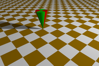
Initially, the top was tilted 1 degree. It begins in a near vertical orientation, but, with a nutation rate of 1 rad/sec.

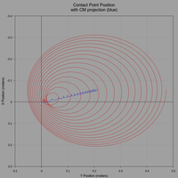
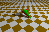
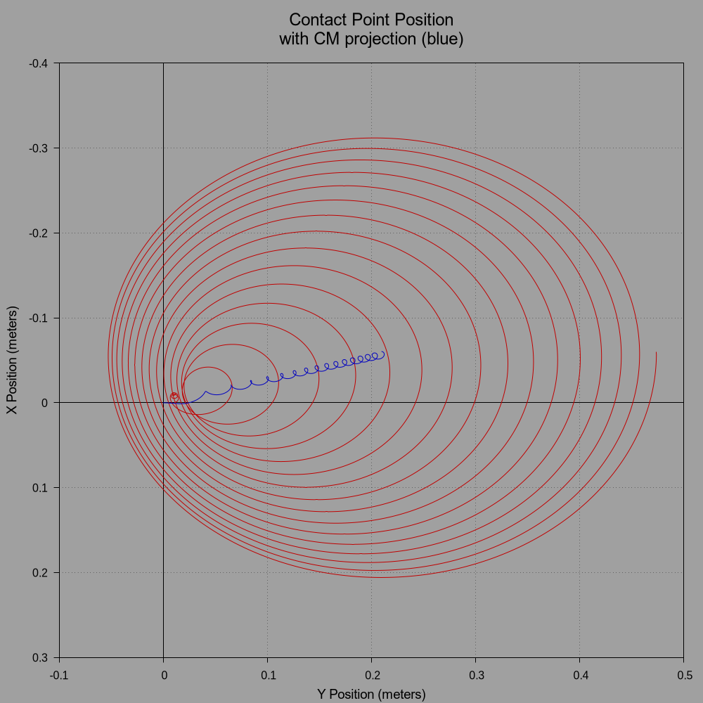
The initial conditions are comparatively mild. The top remains upright until energy loss due to friction causes it to "fall," with the top rotating transversely about the CM as its axis leans more and more to the horizontal. The top seem to defy gravity, but eventually it will intersect the x-y plane and is motion will be disrupted.

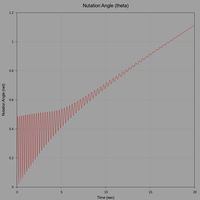
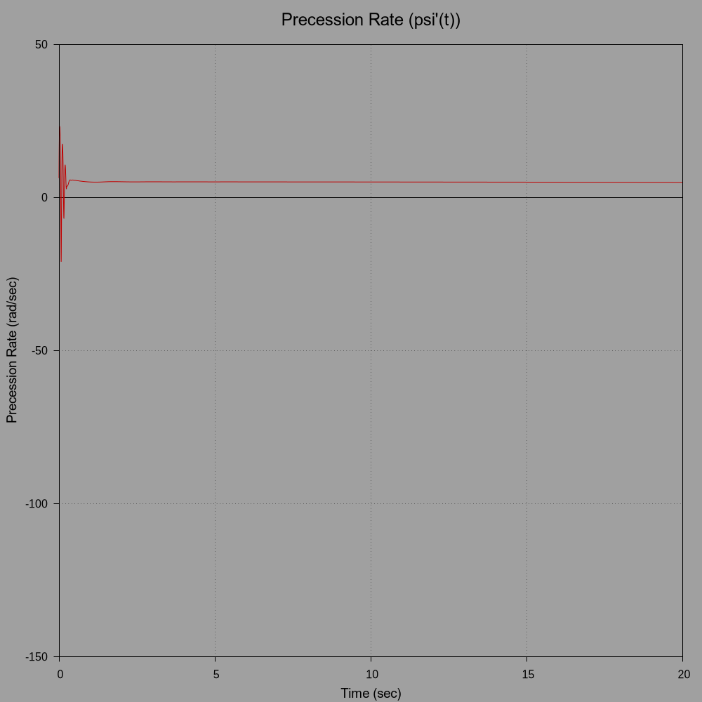
The following plots show the contact point trace with a projection of the CM, precession rate, and nutation angle.

Next is a POV Ray animation of the simulated motion.

Does this simulation reflect reality?

Check out this YouTube video of a real spinning top with similar parameters. The simulated motion is qualitatively identical to this real article.

Note however that the real top in the video is constrained within a concave dish. The simulated top is free to wander but the motion and end result are essentially identical.

We now impart more strenuous initial conditions, in that the nutation rate is 8 times as previous and in the opposite (upward) direction. The top also has a lower initial spin rate and a lower friction coefficient:

ψ = 0 rad
θ = 0.013963 rad
φ = 0 rad
ψ' = 1.28 rad/sec
θ' = -8 rad/sec
φ' = 130 rad/sec
x1 = 0 m
x2 = 0 m
x1' = 0 m/sec
x2' = 0.04 m/sec

The coefficient of kinetic friction is 0.005.

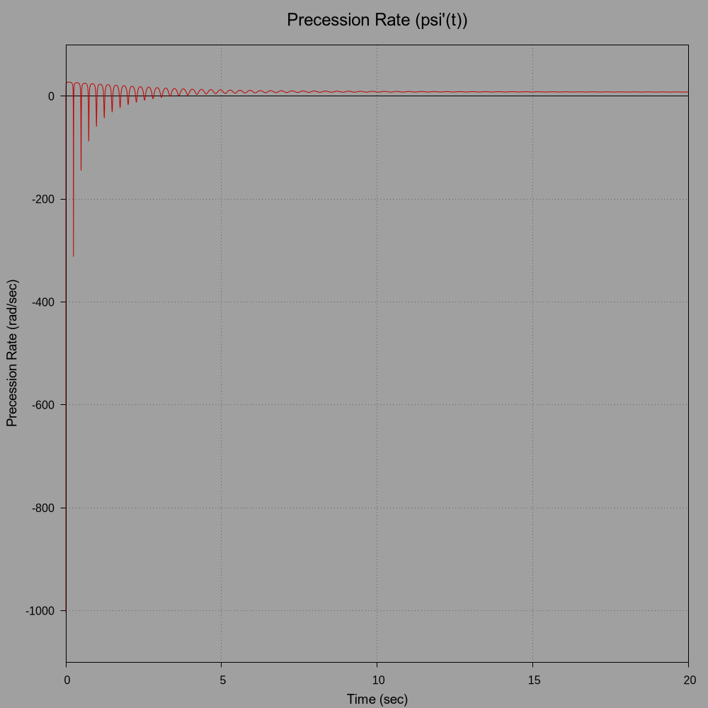
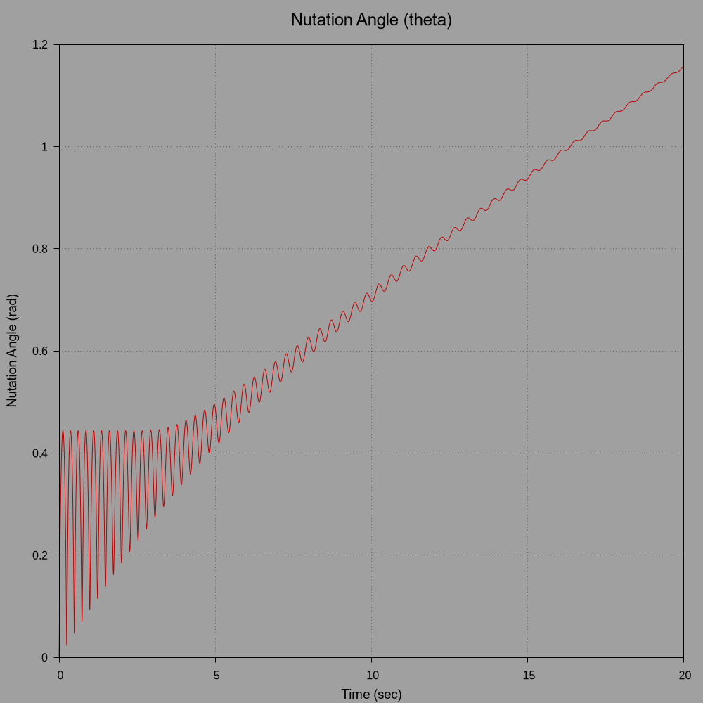
The initial motion is very erratic but stabilizes after 10 seconds. Note how the contact point trace in the following graph reveals the initial unsteady motion. The plot of nutation angle also shows the same. Subsequent motion however, after 10 seconds, is very similar to the previous simulation.

The following plots show the contact point trace with a projection of the CM, precession rate, and nutation angle.

Next is a POV Ray animation of the simulated motion.

The rotation of rigid bodies, to me, is a highly fascinating subject. Although seemingly simple, such rotation requires advanced mathematics for complete explication. Even today, the behavior of mundane objects like bicycles or gyroscopic exercisers have yet to be fully explained mathematically.

Also, this article was intended to display the use of FOSS and GNU/Linux software tools for physical simulations and animation.