The Web Site of L.A.P.

Roulette Curves with GNU/Linux

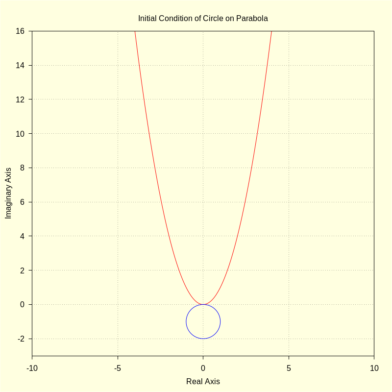
1) A More Complex Example: Circle Rolling on Parabola

The reader should be familiar with the methods outlined in the introductory article on roulettes. Again, we use Maxima/wxMaxima for all derivations.

(%i4)

kill ( all ) $ load ( draw ) $ load ( facexp ) $
assume ( A > 0 , R > 0 , t > = 0 , u > = 0 ) $
set_draw_defaults ( xrange = [ − 10 , 10 ] , yrange = [ − 3 , 16 ] , proportional_axes = xy , grid = true , nticks = 400 ,
background_color = light_yellow , xlabel = "Real Axis" , ylabel = "Imaginary Axis"
) $

The fixed curve is an upward opening parabola with vertex at the origin: y = A * x^2. We express this in complex parameterization:

(%i5)

fx ( t , A ) : = t + %i · A · t ^ 2 ;

\[\operatorname{ }\operatorname{fx}\left( t\operatorname{,}A\right) \operatorname{:=}t+i A {{t}^{2}}\]

Now come the expressions for the derivative and arc length of the fixed curve.

(%i7)

define ( dfx ( t , A ) , diff ( fx ( t , A ) , t ) ) ;
define ( sfx ( t , A ) , integrate ( cabs ( dfx ( t , A ) ) , t ) ) ;

\[\operatorname{ }\operatorname{dfx}\left( t\operatorname{,}A\right) \operatorname{:=}2 i A t+1\]

\[\operatorname{ }\operatorname{sfx}\left( t\operatorname{,}A\right) \operatorname{:=}\frac{\operatorname{asinh}\left( 2 A t\right) }{4 A}+\frac{t \sqrt{4 {{A}^{2}} {{t}^{2}}+1}}{2}\]

The rolling curve, a circle, as complex parameterization with u, and its derivative. We use the polar form instead of the rectangular form.
The circle is centered at (0, -R)
R * exp(i * u/R) - i * R
Factor out i * R

(%i9)

ro ( u , R ) : = %i · R · ( exp ( − %i · u / R ) − 1 ) ;
define ( dro ( u , R ) , ev ( diff ( ro ( u , R ) , u ) , diff ) ) ;

\[\operatorname{ }\operatorname{ro}\left( u\operatorname{,}R\right) \operatorname{:=}i R\, \left( \operatorname{exp}\left( \frac{\left( -i\right) u}{R}\right) -1\right) \]

\[\operatorname{ }\operatorname{dro}\left( u\operatorname{,}R\right) \operatorname{:=}{{e}^{-\frac{i u}{R}}}\]

A plot of the initial conditions of the fixed and rolling curves.

(%i13)

A : 1 $ R : 1 $
wxdraw2d (
   color = red , parametric ( realpart ( fx ( t , A ) ) , imagpart ( fx ( t , A ) ) , t , − 4 , 4 ) ,
   color = blue , parametric ( realpart ( ro ( u , R ) ) , imagpart ( ro ( u , R ) ) , u , 0 , 2 · %pi ) ,
   title = "Initial Condition of Circle on Parabola"
   ) $
kill ( A , R ) $

\[\operatorname{ }\]

We now get the arc length of the rolling curve.

(%i14)

define ( sro ( u , R ) , ev ( integrate ( cabs ( dro ( u , R ) ) , u ) ) ) ;

\[\operatorname{ }\operatorname{sro}\left( u\operatorname{,}R\right) \operatorname{:=}u\]

For the roulette, sro(u,R) = sfx(t,A). We need to solve this equation to get u as a function of t.

(%i15)

define ( ut ( t , R , A ) , rhs ( solve ( sro ( u , R ) = sfx ( t , A ) , u ) [ 1 ] ) ) ;

\[\operatorname{ }\operatorname{ut}\left( t\operatorname{,}R\operatorname{,}A\right) \operatorname{:=}\frac{\operatorname{asinh}\left( 2 A t\right) +2 A t \sqrt{4 {{A}^{2}} {{t}^{2}}+1}}{4 A}\]

We now substitute this expression for u(t) and re-define the rolling curve functions.

(%i18)

logarc : false $
define ( ro ( t , R , A ) , %i · R · ( exp ( − %i · ut ( t , R , A ) / R ) − 1 ) ) ;
define ( dro ( t , R , A ) , ratsimp ( diff ( ro ( t , R , A ) , t ) ) ) ;

\[\operatorname{ }\operatorname{ro}\left( t\operatorname{,}R\operatorname{,}A\right) \operatorname{:=}i R\, \left( {{e}^{-\frac{i \left( \operatorname{asinh}\left( 2 A t\right) +2 A t \sqrt{4 {{A}^{2}} {{t}^{2}}+1}\right) }{4 A R}}}-1\right) \]

\[\operatorname{ }\operatorname{dro}\left( t\operatorname{,}R\operatorname{,}A\right) \operatorname{:=}\sqrt{4 {{A}^{2}} {{t}^{2}}+1} {{e}^{-\frac{i \operatorname{asinh}\left( 2 A t\right) }{4 A R}-\frac{i t \sqrt{4 {{A}^{2}} {{t}^{2}}+1}}{2 R}}}\]

Check to see if the functions and their derivatives at t=0 and equal.

(%i21)

kill ( A , R ) $
fx ( 0 , A ) ;
ro ( 0 , R , A ) ;

\[\operatorname{ }0\]

OK. Initial values are equal.

(%i23)

imagpart ( dfx ( 0 , A ) ) / realpart ( dfx ( 0 , A ) ) ;
imagpart ( dro ( 0 , R , A ) ) / realpart ( dro ( 0 , R , A ) ) ;

\[\operatorname{ }0\]

OK. The first derivative initial values are equal.

Check if the magnitude of the derivatives are equal for t > 0.

(%i25)

cabs ( dfx ( t , A ) ) ;
trigsimp ( cabs ( dro ( t , R , A ) ) ) ;

\[\operatorname{ }\sqrt{4 {{A}^{2}} {{t}^{2}}+1}\]

OK. Everything checks. Let's build the roulettes.

2) Generating the Roulette

All of our functions being defined, we select a generating point, p, and then produce the roulette.

(%i28)

R : 1 $ A : 1 $
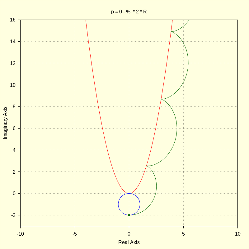
p : 0 − %i · 2 · R ;

\[\operatorname{(p) }-2 i\]

(%i29)

define ( roul ( t ) , fx ( t , A ) + ( p − ro ( t , R , A ) ) · dfx ( t , A ) / dro ( t , R , A ) ) ;

\[\operatorname{ }\operatorname{roul}(t)\operatorname{:=}\frac{\left( 2 i t+1\right) \, \left( -i \left( {{e}^{-\frac{i \left( \operatorname{asinh}\left( 2 t\right) +2 t \sqrt{4 {{t}^{2}}+1}\right) }{4}}}-1\right) -2 i\right) {{e}^{\frac{i \operatorname{asinh}\left( 2 t\right) }{4}+\frac{i t \sqrt{4 {{t}^{2}}+1}}{2}}}}{\sqrt{4 {{t}^{2}}+1}}+i {{t}^{2}}+t\]

(%i30)

wxdraw2d (
   color = red , parametric ( realpart ( fx ( t , A ) ) , imagpart ( fx ( t , A ) ) , t , − 4 , 4 ) ,
   color = blue , parametric ( realpart ( ro ( u , R , A ) ) , imagpart ( ro ( u , R , A ) ) , u , 0 , 2 · %pi ) ,
   color = darkgreen , parametric ( realpart ( roul ( t ) ) , imagpart ( roul ( t ) ) , t , 0 , 4 · %pi ) ,
   point_type = 7 , points [ [ realpart ( p ) ] , [ imagpart ( p ) ] ] ,
   title = "p = 0 - %i * 2 * R"
) $

\[\operatorname{ }\]

Set point p at vertex of parabola.

(%i33)

R : 1 $ A : 1 $
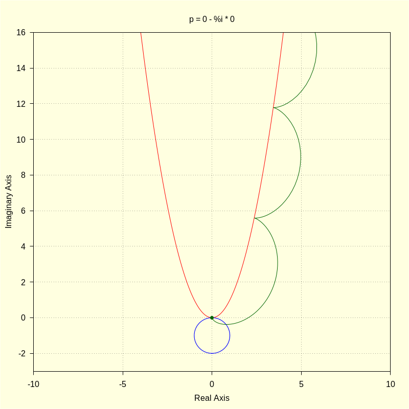
p : 0 − %i · 0 ;

\[\operatorname{(p) }0\]

(%i34)

define ( roul ( t ) , fx ( t , A ) + ( p − ro ( t , R , A ) ) · dfx ( t , A ) / dro ( t , R , A ) ) ;

\[\operatorname{ }\operatorname{roul}(t)\operatorname{:=}-\frac{i \left( 2 i t+1\right) \, \left( {{e}^{-\frac{i \left( \operatorname{asinh}\left( 2 t\right) +2 t \sqrt{4 {{t}^{2}}+1}\right) }{4}}}-1\right) {{e}^{\frac{i \operatorname{asinh}\left( 2 t\right) }{4}+\frac{i t \sqrt{4 {{t}^{2}}+1}}{2}}}}{\sqrt{4 {{t}^{2}}+1}}+i {{t}^{2}}+t\]

(%i35)

\[\operatorname{ }\]

Set point p at center of circle.

(%i38)

R : 1 $ A : 1 $
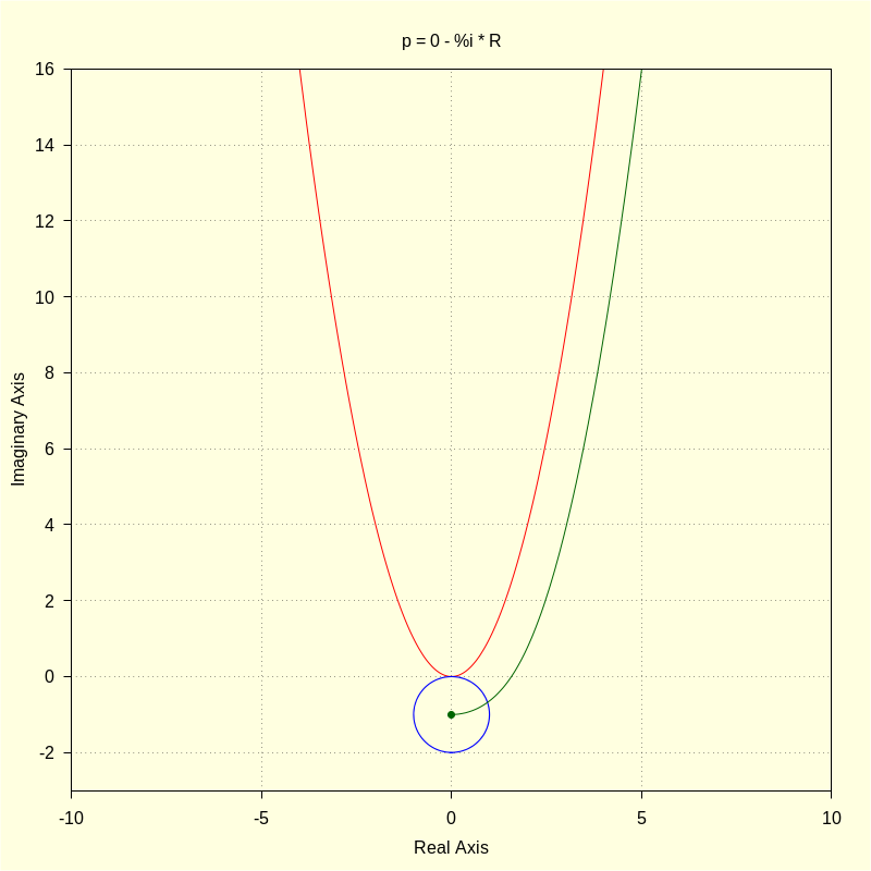
p : 0 − %i · R ;

\[\operatorname{(p) }-i\]

(%i39)

define ( roul ( t ) , fx ( t , A ) + ( p − ro ( t , R , A ) ) · dfx ( t , A ) / dro ( t , R , A ) ) ;

\[\operatorname{ }\operatorname{roul}(t)\operatorname{:=}\frac{\left( 2 i t+1\right) \, \left( -i \left( {{e}^{-\frac{i \left( \operatorname{asinh}\left( 2 t\right) +2 t \sqrt{4 {{t}^{2}}+1}\right) }{4}}}-1\right) -i\right) {{e}^{\frac{i \operatorname{asinh}\left( 2 t\right) }{4}+\frac{i t \sqrt{4 {{t}^{2}}+1}}{2}}}}{\sqrt{4 {{t}^{2}}+1}}+i {{t}^{2}}+t\]

(%i40)

\[\operatorname{ }\]

3) Final Comments

The case of the circle rolling on a parabola illustrates a somewhat complex but still tractable derivation. That is, we can develop analytical expressions for all curves and their derivatives. This however is not always possible as the next examples will show.

Also, the power and convenience of using Maxima/wxMaxima to perform the extensive calculations is nicely demonstrated.

Created with wxMaxima.
Modified and embedded by L.A.P.