The Web Site of L.A.P.

1 Recreational Math: Faster Than Exponential Growth

Are there natural growth rates that are faster than exponential growth? There are certainly many functions that increase faster than the exponential function. For example, this web page gives a few examples thereof, such as the double exponential, the factorial, and the Ackerman function. There is also the Fibonacci function. But such functions seem disjoint and totally unrelated to the exponential function. This article attempts to develop a sequence of functions that are naturally related to the exponential with an arbitrarily faster (and also slower) growth rate.

I should also state at the outset that this article is purely an exercise in recreational mathematics and is not a scholarly endeavor. Mathematics should always be an enjoyable activity for both the professional and the amateur alike.

Furthermore, the importance of the computer algebra system of Maxima/wxMaxima, on a GNU/Linux system, is once again presented. This article is based on a Maxima/wxMaxima worksheet and the reader should have some familiarity with the Maxima syntax, although the derived equations can be self-explanatory. For those interested, the original wxMaxima worksheet is found here.

2 The Exponential Function, $ \exp(t) $, Defined as the Solution to a Differential Equation

The following differential equation defines the exponential function as its solution:

\[ \frac{dx}{dt} = c \cdot x \]

Thus, we can expect a faster growth rate in the variable $x$ if we consider the following modification, with the constant $ k > 1 $:

\[ \frac{dx}{dt} = c \cdot x^k \]

For simplicity, and to adhere to the exponential function behavior, we select $ c = 1 $ with the initial conditions $ x = 1 $ at $ t = 0 $.

Let us first try $ k = 2 $

\[ \frac{dx}{dt} = x^2 \]

2.1 Using Maxima/wxMaxima CAS to Solve the Differential Equation for k = 2

We initialize the Maxima/wxMaxima environment:

-->	killall$ load(draw)$ set_draw_defaults(grid=true, xrange=[0,2], yrange=[0,10], background_color=light_yellow)$

We now define and solve the differential equation at the specified initial conditions:

-->	eqn:'diff(x,t)=x^2; sol:ode2(eqn, x, t); solic:ic1(sol, t=0, x=1); solve(solic, x);

\[ \frac{d}{d t} x\mathop{=}{{x}^{2}}\]

\[ sol: \mathop{-}\left( \frac{1}{x}\right) \mathop{=}t\mathop{+}\ensuremath{\mathrm{\% c}}\]

\[ solic: \mathop{-}\left( \frac{1}{x}\right) \mathop{=}t\mathop{-}1\]

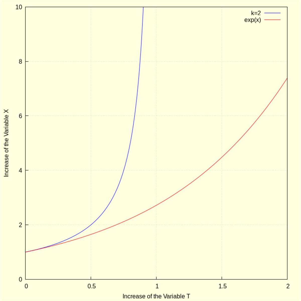
\[ \left[ x\mathop{=}\mathop{-}\left( \frac{1}{t\mathop{-}1}\right) \right] \]

Now we plot the above solution and the exponential function for a visual comparison (click the image for a larger pop-out):

-->	wxdraw2d(key="k=2", explicit(1/(1−t), t,0,2), key="exp(x)", color=red, explicit(exp(t), t,0,2), xlabel="Increase of the Variable T", ylabel="Increase of the Variable X" )$

The solution equation, $ x \mathop{=}-(\frac{1}{(t-1)}) $, shown in blue, does indeed increase much more rapidly than the exponential function (in red). In fact, the solution equation exhibits an asymptote at $ t = 1 $ and will diverge to infinity at this point.

3 The Mathematical Generalization

Mathematics is all about generalization and thus let us develop the general case of the above differential equation with $ k > 1 $ and $x = 1 $ at $ t = 0 $:

\[ \frac{dx}{dt} \mathop{=} x^k \]

Using Maxima/wxMaxima to solve the general case:

-->	assume(k>1)$ eqn:'diff(x,t)=x^k; sol:ode2(eqn, x, t); solic:ic1(sol, t=0, x=1); solve(solic, x);

\[ \frac{d}{d t} x\mathop{=}{{x}^{k}}\]

\[ sol: \mathop{-}\left( \frac{{{x}^{1\mathop{-}k}}}{k\mathop{-}1}\right) \mathop{=}t\mathop{+}\ensuremath{\mathrm{\% c}}\]

\[ solic: \mathop{-}\left( \frac{{{x}^{1\mathop{-}k}}}{k\mathop{-}1}\right) \mathop{=}\frac{\left( k\mathop{-}1\right) \cdot t\mathop{-}1}{k\mathop{-}1}\]

\[ \left[ {{x}^{1\mathop{-}k}}\mathop{=}\mathop{-}\left( k\cdot t\right) \mathop{+}t\mathop{+}1\right] \]

Since $(1 - k) < 0 $ the above expression can be rewritten as:

-->	'x = '1/((t·(1−k)+1)^(1/(k−1)));

\[ x\mathop{=}\frac{1}{{{\left( \left( 1\mathop{-}k\right) \cdot t\mathop{+}1\right) }^{\frac{1}{k\mathop{-}1}}}}\]

From this expression the asymptote is $ \frac{1}{(k-1)} $ as this makes the denominator $ = 0$.

Now, we evaluate the expression at various values of $ k $ and also determine the asymptote:

-->	keq1:ev((−(k·t)+t+1)^(1/(1−k)), k=5); as1:ev(1/(k−1),k=5); keq2:ev((−(k·t)+t+1)^(1/(1−k)), k=2); as2:ev(1/(k−1),k=2); keq3:ev((−(k·t)+t+1)^(1/(1−k)), k=3/2); as3:ev(1/(k−1),k=3/2); keq4:ev((−(k·t)+t+1)^(1/(1−k)), k=10/9); as4:ev(1/(k−1),k=10/9);

\[ keq1: \frac{1}{{{\left( 1\mathop{-}4\cdot t\right) }^{\frac{1}{4}}}}\]

\[ as1: \frac{1}{4}\]

\[ keq2: \frac{1}{1\mathop{-}t}\]

\[ as2: 1\]

\[ keq3: \frac{1}{{{\left( 1\mathop{-}\frac{t}{2}\right) }^{2}}}\]

\[ as3: 2\]

\[ keq4: \frac{1}{{{\left( 1\mathop{-}\frac{t}{9}\right) }^{9}}}\]

\[ as4: 9\]

We now plot the above expressions and limit the range of the t variable by the asymptote. The exponential function $ \exp(t) $, is also plotted for comparison (click the image for a larger pop-out):

-->

wxdraw2d(key="k=5", color=blue, explicit(keq1, t,0,as1),
   key="k=2", color=dark_green, explicit(keq2, t,0,as2),
   key="k=3/2", color=dark_violet, explicit(keq3, t,0,as3),
   key="k=10/9", color=black, explicit(keq4, t,0,as4),
   key="exp(t)", color=red, explicit(exp(t), t,0,2),
   xlabel="Curves Show Decreasing Values (left to right) as the Parameter K ⟶ 1",
   ylabel="Increase of the Variable X"
)$

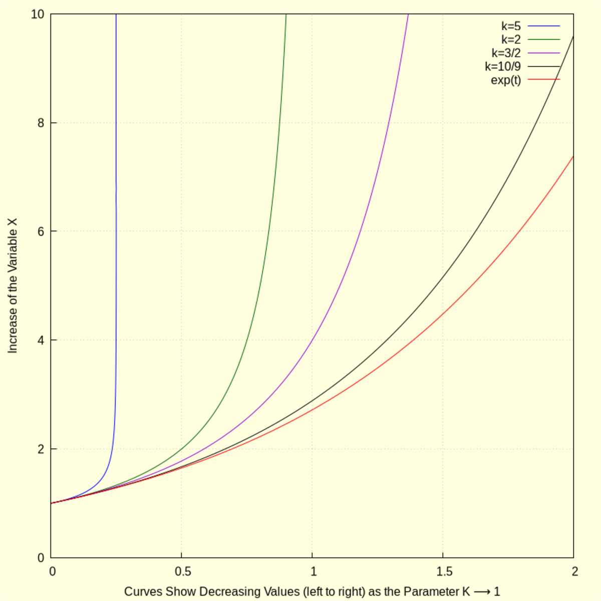
It seems that as the parameter, $ k $, decreases from $ \infty \rightarrow 1 $, the solution equations approach the exponential function $ \exp(t) $.

Let us use Maxima/wxMaxima to determine the limit as $ k \rightarrow 1 $:

-->	limit((−(k·t)+t+1)^(1/(1−k)), k, 1);

\[ {{\% e}^{t}}\]

Indeed. The exponential function is the limit of the sequence.

We have thus determined a whole sequence of functions that increase faster than the exponential function and which are naturally based on the same defining differential equation.

4 Generalization for k < 1

Let us now examine the differential equation solution for values of the exponent being less than $1$. We use the variable $l$ to avoid stepping on the above variable $k$. We expect a slower rate of growth when compared to $\exp(t)$.

-->	assume(l<1)$ eqn:'diff(x,t)=x^l; sol:ode2(eqn, x, t); solic:ic1(sol, t=0, x=1); solve(solic, x);

\[ \frac{d}{d t} x\mathop{=}{{x}^{l}}\]

\[ \mathop{-}\left( \frac{{{x}^{1\mathop{-}l}}}{l\mathop{-}1}\right) \mathop{=}t\mathop{+}\ensuremath{\mathrm{\% c}}\]

\[ \mathop{-}\left( \frac{{{x}^{1\mathop{-}l}}}{l\mathop{-}1}\right) \mathop{=}\frac{\left( l\mathop{-}1\right) \cdot t\mathop{-}1}{l\mathop{-}1}\]

\[ \left[ {{x}^{1\mathop{-}l}}\mathop{=}\mathop{-}\left( l\cdot t\right) \mathop{+}t\mathop{+}1\right] \]

This solution is re-written as:

-->	'x = ((1−l)·t+1)^(1/(1−l));

\[ x\mathop{=}{{\left( \left( 1\mathop{-}l\right) \cdot t\mathop{+}1\right) }^{\frac{1}{1\mathop{-}l}}}\]

We now determine $x(t)$ at several values of $l$:

-->	leq1:ev(((1−l)·t+1)^(1/(1−l)), l=1/10); leq2:ev(((1−l)·t+1)^(1/(1−l)), l=1/2); leq3:ev(((1−l)·t+1)^(1/(1−l)), l=9/10);

\[ leq1: {{\left( \frac{9\cdot t}{10}\mathop{+}1\right) }^{\frac{10}{9}}}\]

\[ leq1: {{\left( \frac{t}{2}\mathop{+}1\right) }^{2}}\]

\[ leq1: {{\left( \frac{t}{10}\mathop{+}1\right) }^{10}}\]

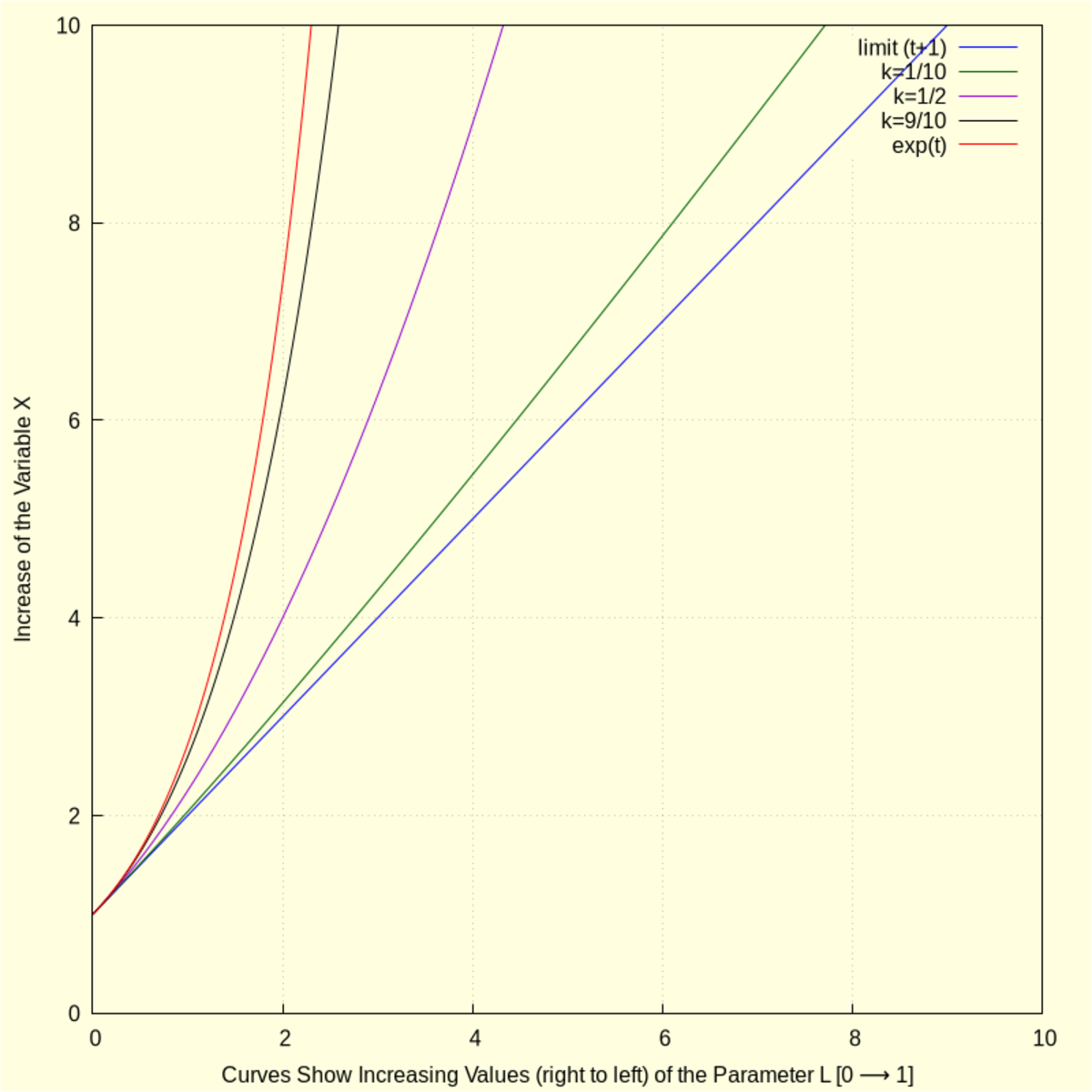
We also note that the limit of this equation as $l \rightarrow 0$ is the linear function $(t + 1)$:

-->	limit(((1−l)·t+1)^(1/(1−l)), l, 0);

\[ t\mathop{+}1\]

The above functions are plotted to compare with $\exp(t)$ (click the image for a larger pop-out):

-->

wxdraw2d(key="limit (t+1)", color=blue, explicit(t+1, t,0,10),
   key="k=1/10", color=dark_green, explicit(leq1, t,0,10),
   key="k=1/2", color=dark_violet, explicit(leq2, t,0,10),
   key="k=9/10", color=black, explicit(leq3, t,0,10),
   key="exp(t)", color=red, explicit(exp(t), t,0,10),
   xrange=[0,10],
   xlabel="Curves Show Increasing Values (right to left) of the Parameter L [0 ⟶ 1]",
   ylabel="Increase of the Variable X")$

A parting check reveals that the limit as $l \rightarrow 1$ is indeed $exp(t)$:

-->	limit(((1−l)·t+1)^(1/(1−l)), l, 1);

\[ {{\% e}^{t}}\]

In this sequence of functions, as the parameter $(k, l)$ varies from $\infty \rightarrow 0$, the exponential function arises $(k = 1)$ as a sort of demarcation between functions with finite asymptotes and functions with asymptotes at $\infty$.

5 A Derivative Check

The derivative of the exponential function, $\exp(t)$, to any order $n$, is equal to $\exp(t)$:

\[ \frac{d^n}{dt^n}\exp(t) = \exp(t) \]

We therefore expect the derivatives of the function sequence $k > 1$, for any order $n$, should converge to $ \exp(t) $ as $k \rightarrow 1$.

Let us use Maxima/wxMaxima to check this for $n = 1 \rightarrow 10 $ (the field below is scrollable horizontally):

-->	eqk:(−(k·t)+t+1)^(1/(1−k))$ for n: 1 thru 10 do ( drv:diff(eqk,t,n), lmt:limit(drv, k, 1), display(n), display(drv), display(lmt) );

\[\]\[n\mathop{=}1 \]\[\ensuremath{\mathrm{Derivative}}\mathop{=}{{\left( \mathop{-}\left( k\cdot t\right) \mathop{+}t\mathop{+}1\right) }^{\frac{1}{1\mathop{-}k}\mathop{-}1}}\]\[\ensuremath{\mathrm{Limit}}\mathop{=}{{\% e}^{t}}\]
\[n\mathop{=}2 \]\[\ensuremath{\mathrm{Derivative}}\mathop{=}\left( \frac{1}{1\mathop{-}k}\mathop{-}1\right) \cdot \left( 1\mathop{-}k\right) \cdot {{\left( \mathop{-}\left( k\cdot t\right) \mathop{+}t\mathop{+}1\right) }^{\frac{1}{1\mathop{-}k}\mathop{-}2}}\]\[\ensuremath{\mathrm{Limit}}\mathop{=}{{\% e}^{t}}\]
\[n\mathop{=}3 \]\[\ensuremath{\mathrm{Derivative}}\mathop{=}\left( \frac{1}{1\mathop{-}k}\mathop{-}2\right) \cdot \left( \frac{1}{1\mathop{-}k}\mathop{-}1\right) \cdot {{\left( 1\mathop{-}k\right) }^{2}}\cdot {{\left( \mathop{-}\left( k\cdot t\right) \mathop{+}t\mathop{+}1\right) }^{\frac{1}{1\mathop{-}k}\mathop{-}3}}\]\[\ensuremath{\mathrm{Limit}}\mathop{=}{{\% e}^{t}}\]
\[n\mathop{=}4 \]\[\ensuremath{\mathrm{Derivative}}\mathop{=}\left( \frac{1}{1\mathop{-}k}\mathop{-}3\right) \cdot \left( \frac{1}{1\mathop{-}k}\mathop{-}2\right) \cdot \left( \frac{1}{1\mathop{-}k}\mathop{-}1\right) \cdot {{\left( 1\mathop{-}k\right) }^{3}}\cdot {{\left( \mathop{-}\left( k\cdot t\right) \mathop{+}t\mathop{+}1\right) }^{\frac{1}{1\mathop{-}k}\mathop{-}4}}\]\[\ensuremath{\mathrm{Limit}}\mathop{=}{{\% e}^{t}}\]
\[n\mathop{=}5 \]\[\ensuremath{\mathrm{Derivative}}\mathop{=}\left( \frac{1}{1\mathop{-}k}\mathop{-}4\right) \cdot \left( \frac{1}{1\mathop{-}k}\mathop{-}3\right) \cdot \left( \frac{1}{1\mathop{-}k}\mathop{-}2\right) \cdot \left( \frac{1}{1\mathop{-}k}\mathop{-}1\right) \cdot {{\left( 1\mathop{-}k\right) }^{4}}\cdot {{\left( \mathop{-}\left( k\cdot t\right) \mathop{+}t\mathop{+}1\right) }^{\frac{1}{1\mathop{-}k}\mathop{-}5}}\]\[\ensuremath{\mathrm{Limit}}\mathop{=}{{\% e}^{t}}\]
\[n\mathop{=}6 \]\[\ensuremath{\mathrm{Derivative}}\mathop{=}\left( \frac{1}{1\mathop{-}k}\mathop{-}5\right) \cdot \left( \frac{1}{1\mathop{-}k}\mathop{-}4\right) \cdot \left( \frac{1}{1\mathop{-}k}\mathop{-}3\right) \cdot \left( \frac{1}{1\mathop{-}k}\mathop{-}2\right) \cdot \left( \frac{1}{1\mathop{-}k}\mathop{-}1\right) \cdot {{\left( 1\mathop{-}k\right) }^{5}}\cdot {{\left( \mathop{-}\left( k\cdot t\right) \mathop{+}t\mathop{+}1\right) }^{\frac{1}{1\mathop{-}k}\mathop{-}6}}\]\[\ensuremath{\mathrm{Limit}}\mathop{=}{{\% e}^{t}}\]
\[n\mathop{=}7 \]\[\ensuremath{\mathrm{Derivative}}\mathop{=}\left( \frac{1}{1\mathop{-}k}\mathop{-}6\right) \cdot \left( \frac{1}{1\mathop{-}k}\mathop{-}5\right) \cdot \left( \frac{1}{1\mathop{-}k}\mathop{-}4\right) \cdot \left( \frac{1}{1\mathop{-}k}\mathop{-}3\right) \cdot \left( \frac{1}{1\mathop{-}k}\mathop{-}2\right) \cdot \left( \frac{1}{1\mathop{-}k}\mathop{-}1\right) \cdot {{\left( 1\mathop{-}k\right) }^{6}}\cdot {{\left( \mathop{-}\left( k\cdot t\right) \mathop{+}t\mathop{+}1\right) }^{\frac{1}{1\mathop{-}k}\mathop{-}7}}\]\[\ensuremath{\mathrm{Limit}}\mathop{=}{{\% e}^{t}}\]
\[n\mathop{=}8 \]\[\ensuremath{\mathrm{Derivative}}\mathop{=}\left( \frac{1}{1\mathop{-}k}\mathop{-}7\right) \cdot \left( \frac{1}{1\mathop{-}k}\mathop{-}6\right) \cdot \left( \frac{1}{1\mathop{-}k}\mathop{-}5\right) \cdot \left( \frac{1}{1\mathop{-}k}\mathop{-}4\right) \cdot \left( \frac{1}{1\mathop{-}k}\mathop{-}3\right) \cdot \left( \frac{1}{1\mathop{-}k}\mathop{-}2\right) \cdot \left( \frac{1}{1\mathop{-}k}\mathop{-}1\right) \cdot {{\left( 1\mathop{-}k\right) }^{7}}\cdot {{\left( \mathop{-}\left( k\cdot t\right) \mathop{+}t\mathop{+}1\right) }^{\frac{1}{1\mathop{-}k}\mathop{-}8}}\]\[\ensuremath{\mathrm{Limit}}\mathop{=}{{\% e}^{t}}\]
\[n\mathop{=}9 \]\[\ensuremath{\mathrm{Derivative}}\mathop{=}\left( \frac{1}{1\mathop{-}k}\mathop{-}8\right) \cdot \left( \frac{1}{1\mathop{-}k}\mathop{-}7\right) \cdot \left( \frac{1}{1\mathop{-}k}\mathop{-}6\right) \cdot \left( \frac{1}{1\mathop{-}k}\mathop{-}5\right) \cdot \left( \frac{1}{1\mathop{-}k}\mathop{-}4\right) \cdot \left( \frac{1}{1\mathop{-}k}\mathop{-}3\right) \cdot \left( \frac{1}{1\mathop{-}k}\mathop{-}2\right) \cdot \left( \frac{1}{1\mathop{-}k}\mathop{-}1\right) \cdot {{\left( 1\mathop{-}k\right) }^{8}}\cdot {{\left( \mathop{-}\left( k\cdot t\right) \mathop{+}t\mathop{+}1\right) }^{\frac{1}{1\mathop{-}k}\mathop{-}9}}\]\[\ensuremath{\mathrm{Limit}}\mathop{=}{{\% e}^{t}}\]
\[n\mathop{=}10 \]\[\ensuremath{\mathrm{Derivative}}\mathop{=}\left( \frac{1}{1\mathop{-}k}\mathop{-}9\right) \cdot \left( \frac{1}{1\mathop{-}k}\mathop{-}8\right) \cdot \left( \frac{1}{1\mathop{-}k}\mathop{-}7\right) \cdot \left( \frac{1}{1\mathop{-}k}\mathop{-}6\right) \cdot \left( \frac{1}{1\mathop{-}k}\mathop{-}5\right) \cdot \left( \frac{1}{1\mathop{-}k}\mathop{-}4\right) \cdot \left( \frac{1}{1\mathop{-}k}\mathop{-}3\right) \cdot \left( \frac{1}{1\mathop{-}k}\mathop{-}2\right) \cdot \left( \frac{1}{1\mathop{-}k}\mathop{-}1\right) \cdot {{\left( 1\mathop{-}k\right) }^{9}}\cdot {{\left( \mathop{-}\left( k\cdot t\right) \mathop{+}t\mathop{+}1\right) }^{\frac{1}{1\mathop{-}k}\mathop{-}10}}\]\[\ensuremath{\mathrm{Limit}}\mathop{=}{{\% e}^{t}}\]

Indeed. In each case the limit of the derivative as $k \rightarrow 1$ converges to $\exp(t)$.

6 Final Comment

The above has been purely a recreational undertaking but it hopefully reveals the utility of the Maxima/wxMaxima CAS to remove the tedium of mathematical derivation and thus to permit an unburdensome exploration. I did not once put a pencil to paper.

Created with wxMaxima.
Modified and embedded by L.A.P.