A Chaos (Nonlinear Dynamics) Demo with GNU/Linux
The incredible success of Newtonian physics and the Calculus in the 17th and 18th centuries, especially as they formed the underpinning of the industrial revolution, led the famed scientist Pierre-Simon Laplace to propose that an absolute determinism was possible, if only in principle. This idea, known as Laplace's demon, assumes that by knowing the present position and velocity of all particles at a given time the entirety of the future and the past can be completely determined.
Absolute determinism, from the perspective of classical mechanics, does indeed seem compelling, but the subsequent development of thermodynamics in the 19th century and later the revolutionary quantum mechanics in the 20th century has essentially given a death blow to the concept of scientific determinism. The universe, as these later theories revealed, can only be certain in a statistical, and not an absolute, sense.
However, even within classical mechanics itself there arose a phenomenon that destroyed the hope of ever knowing the future (and past) by knowing the present. That phenomenon is known as chaos, and it is chaos that ensures that an absolutely deterministic system can be absolutely unpredictable.
In this article, the emergence of chaotic behavior in a simple mechanical system, and the consequences thereof, as shown with GNU/Linux software tools, will be explored.
As usual in this website, although the topics can be quite mathematically complex, I cannot devote the time and space to provide a comprehensive background. The reader should avail himself of the existing material on chaos, or non-linear dynamics as it is properly called, that is widely available on the web or elsewhere. Furthermore, although the discussion presented here will not be overly sophisticated, it is also assumed that the reader has at least an undergraduate-level understanding of physics and mathematics.
The System
Chaos arises from the non-linearity of natural laws, and that is why the subject is often known as non-linear dynamics.
We will consider the case of a simple oscillator (e.g. a spring) that can be modelled in a completely linear and hence completely deterministic fashion using Hooke's Law:
\[ \frac{d^2x}{dt^2} = -\frac{k}{m} * x \](m is the mass and K is a stiffness constant)
This second-order differential equation gives a pure analytical solution that will describe the motion, or state, of the system for all time.
However, if we introduce a non-linear restoring force, which more closely models real-world behavior, the solution becomes analytically intractable:
\[ m * \frac{d^2x}{dt^2} = -k * x + b * x^3 \](b is the non-linear coefficient)
For an even better model of the real world, we need to also include a damping term, a function of velocity, that serves to dissipate energy and a forcing term which produces energy:
\[ m * \frac{d^2x}{dt^2} = -c * \frac{dx}{dt} -k * x + b * x^3 + d * cos(\omega t) \](c is the damping coefficient and d is the amplitude of the forcing)
The above equation is known as the Duffing equation and it is known to give rise to chaotic behavior. Many scholarly volumes have been written about the Duffing equation which underscores its fundamental importance.
The Path to Chaos
To understand how chaos can arise in this simple system we need to examine the potential energy profile, \( U(x) \):
\[ U(x) = \int -k*x + b*x^3\, \mathrm{d}x = -k * \frac{x^2}{2} + b * \frac{x^4}{4} \]Setting k and b equal to unity a graphical plot, using gnuplot, of this profile now follows:

(click to view full size)
The potential energy has a double-well shape. There are two points, or essentially two regions, of minimum energy. Depending upon the magnitude of the driving force, \(d\), and the other system parameters, the system can remain in either region or it can "hop" between regions. It is this potential for "hopping" that leads to chaotic behavior.
Given sufficient time, a mechanical system, after the initial, or transient, response decays, will settle into one of four types of phase-space "orbits:"
- 1. Single point
- 2. Limit cycle
- 3. Quasi-Periodic motion 4. Chaos (really, none of the above)
The primary concern of this article is the emergence of chaos, but we will also show some limit cycles of the system for the purpose of contrast and because a "period doubling" of the limit cycles will often precede chaos.
The Solution Method and an Initial Caveat
To solve the Duffing equation, which is second order, we rewrite it as a system of two first-order differential equations:
\[ \begin{array}{lcl} \displaystyle\frac{dx}{dt} & = & v \\ \displaystyle\frac{dv}{dt} & = & -c * \displaystyle\frac{dx}{dt} -k * x + b * x^3 + d * cos(\omega t) \end{array} \]Thus, the state variables of the system are the position, \(x\), and the velocity, \(v\).
At this point, the informed reader may know that chaos is not possible in a mechanical system that has less than 3 variables. So how can we expect chaos to arise with a two-variable system?
Our system is actually a non-autonomous system. That is, the second equation depends explicitly on time, \(t\).
We can again rewrite the system by defining a third variable, \( z = \omega*t \):
\[ \begin{array}{lcl} \displaystyle\frac{dx}{dt} & = & v \\ \displaystyle\frac{dv}{dt} & = & -c * \displaystyle\frac{dx}{dt} -k * x + b * x^3 + d * cos(z) \\ \displaystyle\frac{dz}{dt} & = & \omega \end{array} \]
Now we have an autonomous, three-variable system where there is no dependence on time and hence we can expect chaos to arise.
However, to keep the graphics simple we shall retain the two-variable form, except to clarify a point on limit cycles as seen below. But keep in mind that all 2D plots are essentially a projection of the 3D phase space.
GNU/Linux Software Tools
The GNU/Linux FOSS software used is listed here:
- GSL: The workhorse of this article is GSL. The Duffing equation system is numerically integrated
at various driving magnitudes using the implicit Runge-Kutta ODE solver.
- Gnuplot: A versatile plotting package.
- ImageMagick: Utilities for image processing.
- Ffmpeg: Creation of the video animations from gnuplot still images.
- Bash: The standard GNU/Linux scripting language used to automate most of the processing.
Results and the Emergence of Chaos
The prime characteristic of chaos is the sensitive dependence on initial conditions. A very small change in the value or certainty of an initial parameter can lead to a drastic divergence of the resulting system trajectory. It is this characteristic that causes a completely deterministic system, as defined by a differential equation system, to exhibit essentially randomness and unpredictability.
In the examples that follow, we demonstrate how the same mechanical system can express both extreme stability and chaos with a simple alteration of parameters.
All system parameters are set to unity, except the driving frequency which is fixed at 1.4 rad/sec. Only the driving amplitude, \( d \), is varied. The initial conditions are always \( x_0 = 1 \), \( v_0 = 0 \).
Ample time was given for each solution to reach some sort of steady state following the transient decay. The interest is in the asymptotic behavior of the system. The exact time will be noted for each example below. The asymptotic behavior is plotted using the final 1000 data points of the numerical solution.
For all of the gritty technical details, the reader can examine the GSL C program which I wrote for these simulations.
1. A Single-Period Limit Cycle
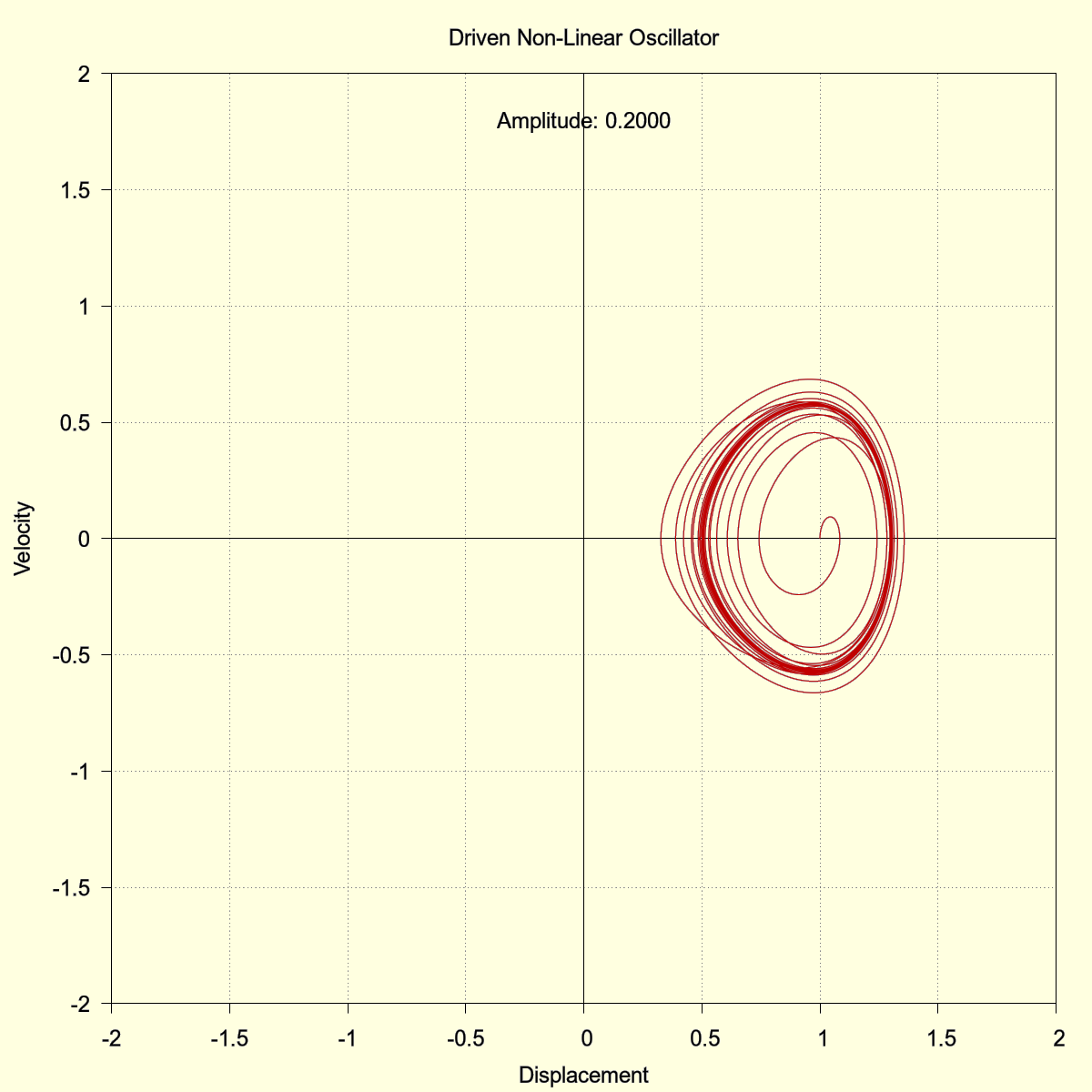
At a driving amplitude of 0.2000 the system settles into a single-period limit cycle. The run time of the simulation was 2000 seconds with time steps of 0.01 second. The other initial parameters are as described above.
Note how in the following image the transient response decays and the phase-space trajectory tightens into a limit cycle.
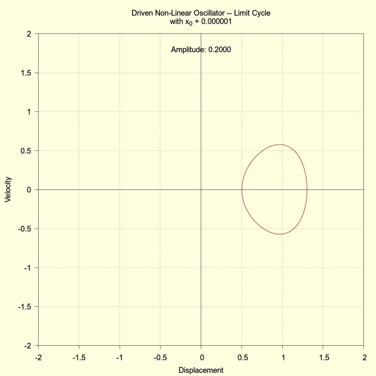
In the subsequent two plots only the final time steps are plotted which clearly reveals the single-phase limit cycle.
The plot on the right shows the same simulation but with the initial vale \( x_0 \) incremented by 0.00001. The resulting limit cycle is identical (to within 3 decimal places after 2000 seconds) to the plot on the left which indicates that there is no sensitivity to changing initial conditions, at least not at this small level. But this small change will make a difference when the system becomes chaotic, as we will see below.
(click to view full size)

(click to view full size)
(click to view full size)
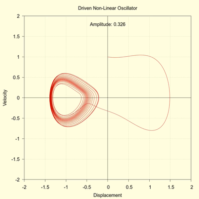
2. A 2-Period Limit Cycle
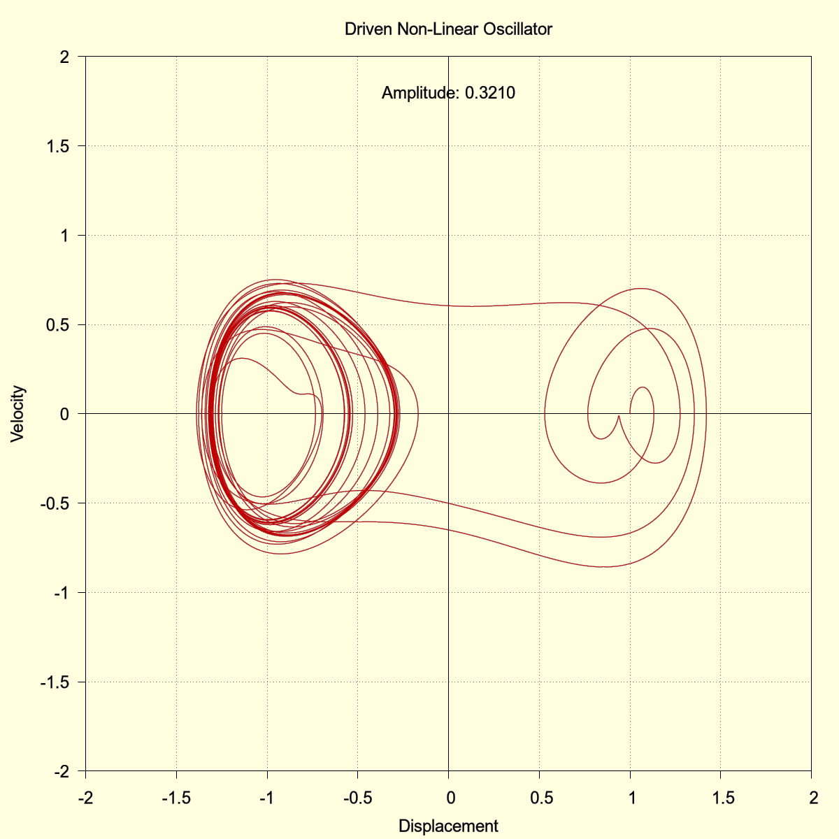
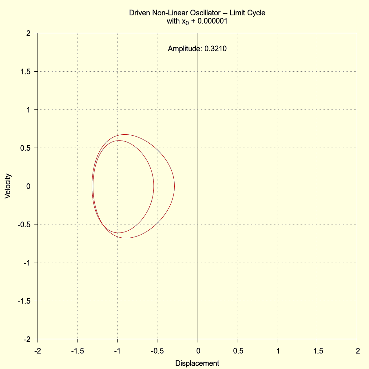
The path to chaos will frequently involve period doubling, and as we increase the driving amplitude to 0.3210 this is exactly what we observe.
The following images show the same sequence as the previous. First, the entire 8000 second time range is plotted which reveals the system transient response. But note how the system trajectory, which begins at \( x_0 = 1 \) now shifts into the negative displacement region. This behavior corresponds to the "hopping" between the potential energy wells as mentioned above. The system has essentially "hopped" into a different potential well but it becomes trapped in this other well as the transient response decays and the system trajectory tightens into another stable limit cycle.
(click to view full size)
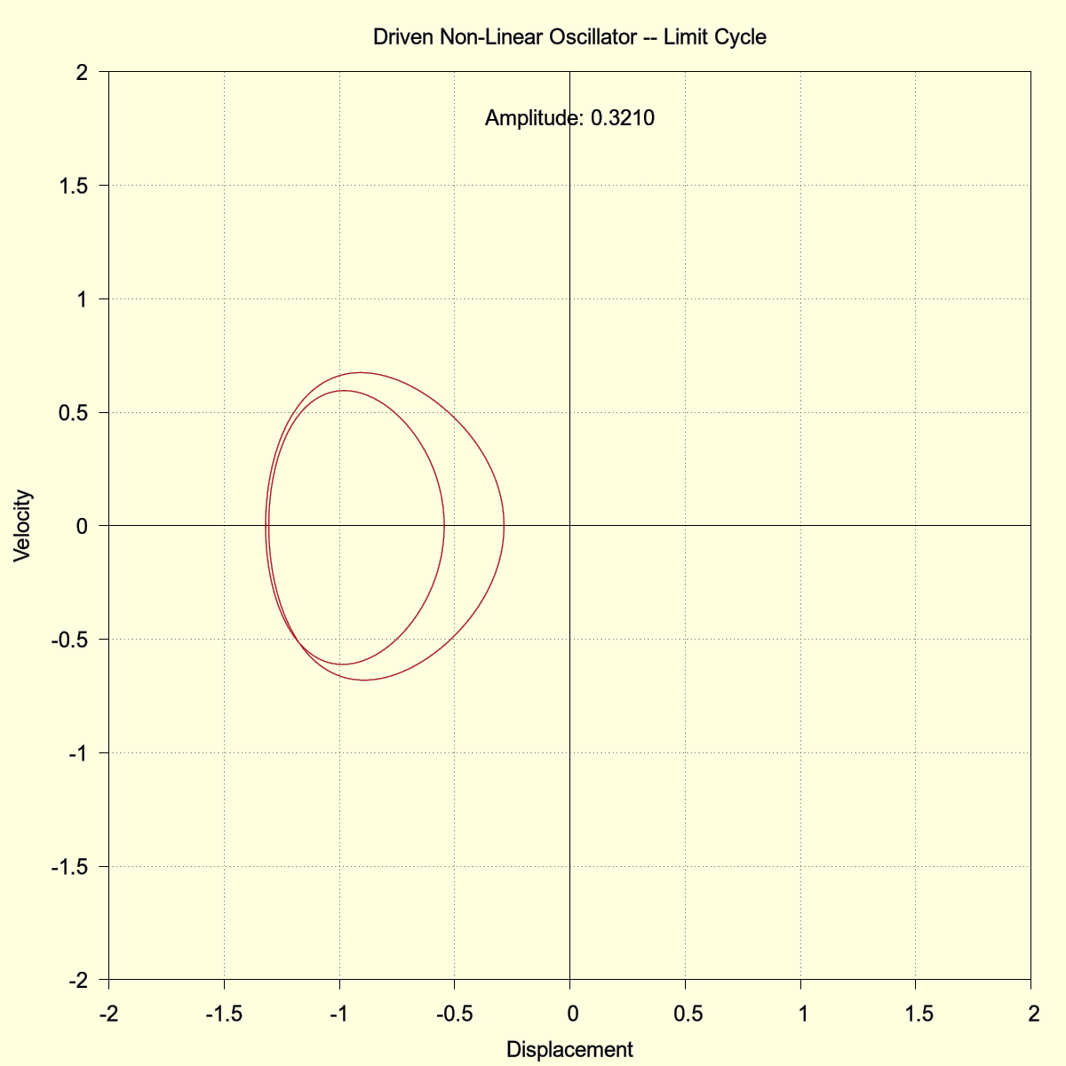
The next images, however, show that this limit cycle has a double period, and again, the right image shows that a small change in the initial condition leads to the same cycle (to within 3 decimal places after 8000 seconds). There is no chaotic behavior here.
(click to view full size)
(click to view full size)
The informed reader may understand that phase-space trajectories do not ever intersect, yet the above images of the limit cycle do show an intersection. But this is merely an artifact of our two-variable, non-autonomous system. If we utilize the three-variable, autonomous system, as described above, the phase-space trajectories never intersect as shown in the following image.

(click to view full size)
Essentially, all two-variable plots shown in this article are a parallel projection of the associated three-variable system.
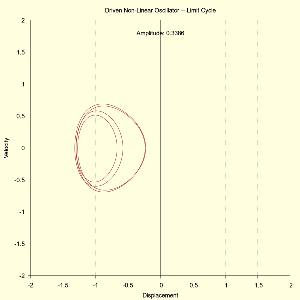
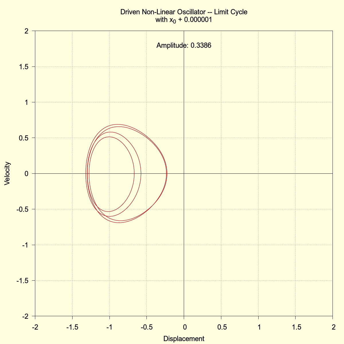
3. A 4-Period Limit Cycle
The driving amplitude is increased to 0.3386 and the run time now is extended to 8000 seconds. The phase space plot seems a tangled mess as the system hops between the potential wells. But the following two images, which plot only the final 2000 seconds, reveal that the system eventually settles into a stable limit cycle. Again, this is not chaos.
(click to view full size)
(click to view full size)
(click to view full size)
The period has doubled from the previous 2-cycles to 4-cycles. Furthermore, as the right image clearly shows, perturbing the initial condition results in the same stable limit trajectory (to within 3 decimal places after 8000 seconds). The system is not chaotic.
4. Chaos At Last
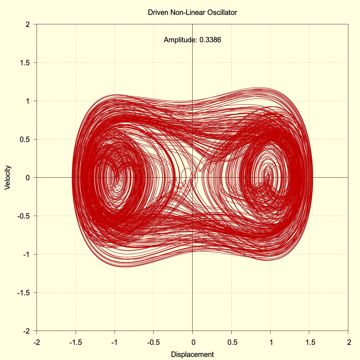
The driving frequency now becomes 0.4000 and the run time is again 8000 seconds. The trajectory demonstrates the same repetitive hopping between the potential wells as seen previously. At the scale of this image the trajectories are so bunched together that in some areas they become fused into a continuous mass. But this is only an artifact of the digital plot. The following two images examine the last 2000 seconds, which should reveal any stable system trajectory.

(click to view full size)
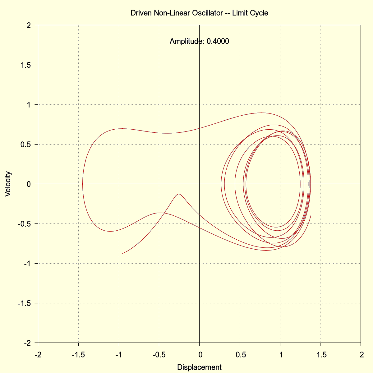
(click to view full size)

(click to view full size)
The system apparently has not settled into any kind of stable state. The run time could be extended indefinitely and only a continual unsteady hopping would likely be observed. The system is definitely in a chaotic state. As the right image shows, a very small increase in the initial condition (1.0E-5) leads to a drastic change in the trajectory. This sensitivity to initial conditions is one of the hallmarks of chaos.
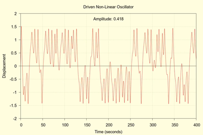
Exploration Through Animation
What follows are animations (i.e. videos) showing two different "views" of the system over a range of driving amplitudes. The first video shows the phase plot of system variables, namely displacement and velocity. The second video shows the system as a plot of displacement versus time. This view is less abstract and depicts what would actually be directly observed.
As the driving amplitude is swept upward from 0.200 to 0.999 the system will experience bouts of chaos that are seemingly interspersed with regions of stability. The following two animations show this behavior.
(click to view video)
(click to view video)
Although the run time for each animation "frame" is only 400 seconds, this time is sufficient to discern the development of a stable state or a chaotic state.
The initial condition are similar to those of the above simulations but not identical with the main difference being the initial conditions: \( x_0=0, v_0=1 \). In spite of these changes the system enters the first region of chaos at about the same driving amplitude of 0.382
Conclusions
It is a non-linear world. This undeniable fact precludes knowing the future (and the past) by knowing the present.
What does it mean "to know?" We can only know by measuring and defining initial conditions, yet even the very best of our measurements are valid to only four or five decimal places. In the above demos we have seen how comparable perturbations can drastically alter future trajectories. The universal character of non-linearity will forever thwart our ability to completely anticipate the future.
References
The topic of non-linear dynamics, or chaos, is enormous and I am certainly no expert. For this humble article I have relied mainly on two excellent references:
Of course there are many more references to be found on the Internet or in public/university libraries. All readers are encouraged to explore on their own this fascinating subject of chaos and its implications. Highly effective GNU/Linux tools are always available to aid in any quest for further understanding.