The Web Site of L.A.P.

Atomic Orbital Plotting with GNU/Linux

Quantum Mechanics is a vast subject that cannot be considered, in even an elementary fashion, within this article. My purpose here is to demonstrate the use of GNU/Linux software tools in the visualization and plotting of atomic orbitals. A sufficient background in quantum mechanics is assumed of the reader. Also, it is not my intention to provide a virtual museum of AO shapes as is usually found on the web. Rather I will develop a general method of deriving and plotting atomic orbitals, illustrated by only a few simple and complex examples, that any interested reader can duplicate.

1 What is an atomic orbital (AO)?

The electrons bound within an atom by the electrical potential of the nucleus are best described not as point particles but as extended waves, which in this case are matter waves (link1, link2). The actual position of the electron, or more accurately the probability thereof, is given by the square (really the complex conjugate) of the function that describes this matter wave. An atomic orbital is a visual depiction of this probability density in space.

The matter wave functions derive from the Schroedinger equation and are only approximations to the real behavior, and spatial location, of electrons. The Schroedinger equation does not account for either the "spin" angular momentum of the electron or relativistic effects. However, to obtain a basic, qualitative grasp of many atomic properties and behavior the atomic orbital picture arising from the Schroedinger equation is very useful.

We begin by providing a quick mathematical background of the Schroedinger equation (SE) and its solution as it is applied to a one-electron, hydrogen-like atom.

2 The Schroedinger Equation (Time Independent)

All derivations are accomplished with the Maxima/wxMaxima package and the reader should be familiar with the syntax, which although straightforward can be at times a bit arcane.

-->	funmake ( Ψ , [ x , y , z ] ) $ − ħ ^ 2 / ( 2 · m ) · ( diff ( Ψ ( x , y , z ) , x , 2 ) + diff ( Ψ ( x , y , z ) , y , 2 ) + diff ( Ψ ( x , y , z ) , z , 2 ) ) + V ( x , y , z ) · Ψ ( x , y , z ) = E · Ψ ( x , y , z ) ;

\[\operatorname{ }\operatorname{V}\left( x\operatorname{,}y\operatorname{,}z\right) \operatorname{\Psi }\left( x\operatorname{,}y\operatorname{,}z\right) -\frac{\left( \frac{{{∂}^{2}}}{∂ {{z}^{2}}} \operatorname{\Psi }\left( x\operatorname{,}y\operatorname{,}z\right) +\frac{{{∂}^{2}}}{∂ {{y}^{2}}} \operatorname{\Psi }\left( x\operatorname{,}y\operatorname{,}z\right) +\frac{{{∂}^{2}}}{∂ {{x}^{2}}} \operatorname{\Psi }\left( x\operatorname{,}y\operatorname{,}z\right) \right) {{\hbar }^{2}}}{2 m}=E \operatorname{\Psi }\left( x\operatorname{,}y\operatorname{,}z\right) \]

The SE is a partial differential equation, essentially a wave equation, shown above in Cartesian coordinates, the solution of which describes a wave in terms of time and/or position variables. In this case, the wave, Ψ(x,y,z), is a matter wave.

Solving the SE is complex but in the case of a one-electron, hydrogen-like atom it is exact. Since the mathematical details are not necessary for this article I will just provide a quick outline.

1) The SE is expressed in spherical coordinates, (r, θ, φ), which are most appropriate for an atomic system, where it becomes separable. For the case of a one-electron, hydrogen-like atom the potential energy is $ V(r) = e^{\frac{2}{r}} $, where e is the electron charge.

2) The solution, Ψ, is therefore the product of the separated functions in the variables:

Ψ(r, θ, φ) = R(r) * Y(θ, φ), i.e. a radial function and an angular function.

The quantum numbers, n, l, m, which define an atomic state, arise from the fact that both the radial and angular functions are expressed, in part, as polynomials which can only exist with certain integral parameters. These parameters then become the quantum numbers. In fact, the angular solution, Y(θ, φ), is nothing more than the ordinary spherical harmonics.

More depth and details are here: http://hyperphysics.phy-astr.gsu.edu/hbase/quantum/hydsch.html

The complete solutions are provided here as a reference for the plotting routines that follow. Each solution depends on the quantum numbers shown in the subscript.

2.1 The Radial Component of the SE Solution

-->	R_nl ( r ) : = ρ ^ ( 3 / 2 ) · sqrt ( ( n − l − 1 ) ! / ( 2 · n · ( ( n + l ) ! ) ) ) · exp ( − ρ · r / 2 ) · ( ρ · r ) ^ l · L ( ρ · r ) ;

\[\operatorname{ }\operatorname{R\_ nl}(r)\operatorname{:=}{{\rho }^{\frac{3}{2}}} \sqrt{\frac{\left( n-l-1\right) \operatorname{!}}{2 n\, \left( n+l\right) \operatorname{!}}} \operatorname{exp}\left( \frac{\left( -\rho \right) r}{2}\right) {{\left( \rho r\right) }^{l}} \operatorname{L}\left( \rho r\right) \]

Here, $ \rho=\frac{2*Z}{n*a0} $, Z = atomic number, a0 = 0.529 Å (Bohr radius). Since for plotting purposes we can use Z=1, this reduces to the nice approximation of ρ = 4/n.

L(ρ*r) is the associated (generalized) Laguerre polynomial and depends on the quantum numbers n, l.

Note that R(r) is a real-valued function in r.

2.2 The Angular Component of the SE Solution

-->	Y_ml ( θ , φ ) : = %i ^ ( m + abs ( m ) ) · sqrt ( ( 2 · l + 1 ) / ( 4 · %pi ) ) · sqrt ( ( l − abs ( m ) ! ) / ( l + abs ( m ) ! ) ) · P · ( cos ( θ ) ) · %e ^ ( %i · m · φ ) ;

\[\operatorname{ }\operatorname{Y\_ ml}\left( \theta \operatorname{,}\phi \right) \operatorname{:=}{{i}^{m+\left| m\right| }} \sqrt{\frac{2 l+1}{4 \ensuremath{\pi} }} \sqrt{\frac{l-\left| m\right| \operatorname{!}}{l+\left| m\right| \operatorname{!}}} P \cos{\left( \theta \right) } {{e}^{i m \phi }}\]

Here, P is the associated Legendre polynomial in the variable cos(θ), and it depends on quantum numbers l, m.

Note that Y(θ, φ) is a complex-valued function in θ, φ.

3 The Background on Plotting the Atomic Orbitals

Maxima/wxMaxima is used to determine the radial and angular wave functions based on a set of quantum numbers. This computer algebra software (CAS) does all of the (very) heavy lifting. Without it, deriving the equations would be a tedious and painstaking task. Maxima/wxMaxima is also used to construct the initial angular and radial probability density plots.

Geomview with StageTools is then used to create a plot and optional animations to allow a fuller appreciation of the AO "shapes."

Keep in mind that AO plots are actually 4-dimensional, that is the value of the wave function depends on 3 spatial coordinates: Ψ = Ψ(r, θ, φ). Such functions cannot be plotted in 3-D space. Therefore the AO can only be visualized by taking a 3-D "slice" at a particular value of the probability density.

We shall consider first the angular probability density which, because it depends only on two variables, θ and φ, can be directly visualized. However this plot does not provide a true indication of orbital shape because the angular density is modulated by the radial density function which can contain "nodes" or points where the wave function (and concommitant probability) is zero.

Secondly, the radial density function is presented as a 2-D plot since only a single variable, r, is involved.

Lastly, the two plots are combined (multiplied) to reveal the true orbital picture. The initial plot will consist of contours at select values of probability density. This is accomplished by eliminating the φ variable due to spherical symmetry. Then, at a single value of probability density a surface of rotation will be created to depict the "true" orbital shape (but see the caveat below).

It is important to note that most textbooks on atomic orbitals, and especially chemistry texts, do not plot the actual complex-valued solutions of the SE. Rather, real-valued solutions are obtained through linear combinations of the complex wave functions.

We shall not follow this common approach. Although such real-valued functions are perfectly valid solutions to the SE they contain "superpositions" and cannot in many cases be given a definite value of the m quantum number. To ensure that each AO picture is based on a definite set of quantum numbers we will use only the complex-valued solutions of the SE.

4 Plotting the Atomic Orbitals

We use Maxima/wxMaxima to develop a routine that will provide all the necessary functions for a given set of quantum numbers, n, l, and m.

It should be noted that the complex portion of the angular function, $ e^{i m φ} $, when squared by multiplying by the complex conjugate, equals 1 for any m. As a consequence, it will always be omitted from the following calculations.

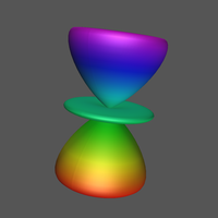
4.1 Quantum Numbers n=2, l=0, and m=0.

The first, simple, example will use n=2, l=0, and m=0. This AO is commonly known as the 2s orbital although the precise designation would be Ψ_200.

A lot of background information will be provided with this first example that will be omitted from subsequent examples.

-->	kill ( all ) $ load ( orthopoly ) $ load ( draw ) $

-->	set_draw_defaults ( xu_grid = 100 , yv_grid = 100 , nticks = 100 , background_color = light_yellow , ip_grid = [ 100 , 100 ] , ip_grid_in = [ 100 , 100 ] , xlabel = "Bohr Radius Units" ) $

-->

n : 2 $ l : 0 $ m : 0 $
coeff : %i ^ ( m + abs ( m ) ) · sqrt ( ( ( l − abs ( m ) ) ! ) / ( ( l + abs ( m ) ) ! ) ) · sqrt ( ( 2 · l + 1 ) / 4 / %pi ) $
P_lm : expand ( assoc_legendre_p ( l , abs ( m ) , cos ( θ ) ) ) $
define ( aprob ( θ , φ ) , ( coeff · P_lm ) ^ 2 ) ;
/* calculate radial probability */
a : n − l − 1 $ b : 2 · l + 1 $ ρ : 4 / n $
L : expand ( sum ( ( ( a + b ) ! ) / ( ( k + b ) ! ) / ( ( a − k ) ! ) / ( k ! ) · ( − r · ρ ) ^ k , k , 0 , a ) · ρ ^ l · r ^ l ) $
Rcoeff : ρ ^ ( 3 / 2 ) · sqrt ( ( ( n − l − 1 ) ! ) / ( 2 · n ) / ( ( n + l ) ! ) ) · exp ( − ρ · r / 2 ) $
define ( rprob ( r ) , ( L · Rcoeff ) ^ 2 ) ;

\[\operatorname{ }\operatorname{aprob}\left( \theta \operatorname{,}\phi \right) \operatorname{:=}\frac{1}{4 \pi }\]

\[\operatorname{ }\operatorname{rprob}(r)\operatorname{:=}{{\left( 2-2 r\right) }^{2}} {{e}^{-2 r}}\]

Because these functions express probability density, their integral over the entire appropriate coordinate intervals must equal 1, i.e. they must be "normalized." This section is a check for this normalization.

-->

/* check for normalization */
' integrate ( rprob ( r ) · r ^ 2 , r , 0 , inf ) ; integrate ( rprob ( r ) · r ^ 2 , r , 0 , inf ) ;
inner_int : ' integrate ( aprob ( θ , φ ) · sin ( θ ) , θ , 0 , %pi ) $
' ( integrate ( ' ' inner_int , φ , 0 , 2 · %pi ) ) ;
integrate ( integrate ( aprob ( θ , φ ) · sin ( θ ) , θ , 0 , %pi ) , φ , 0 , 2 · %pi ) ;

\[\operatorname{ }\int_{0}^{\infty }{\left. {{\left( 2-2 r\right) }^{2}} {{r}^{2}} {{e}^{-2 r}}dr\right.}\]

\[\operatorname{ }1\]

\[\operatorname{ }\int_{0}^{2 \ensuremath{\pi} }{\left. \frac{\int_{0}^{\ensuremath{\pi} }{\left. \sin{\left( \theta \right) }d\theta \right.}}{4 \ensuremath{\pi} }d\phi \right.}\]

\[\operatorname{ }1\]

4.1.1 Angular Probability Density

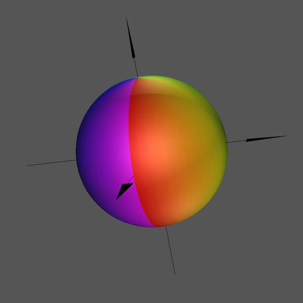
The angular probability is plotted with Geomview/StageTools using the above Maxima-derived equation. The coloration of the surface corresponds to the phase angle, φ, although it is not terribly significant in this context. Here, the color merely enables the spherical property to be better discerned. Because a sphere has no orientation features a set of coordinate axes has been added. Click on the image to bring up a short Ogg video animation.

Click Image for Video

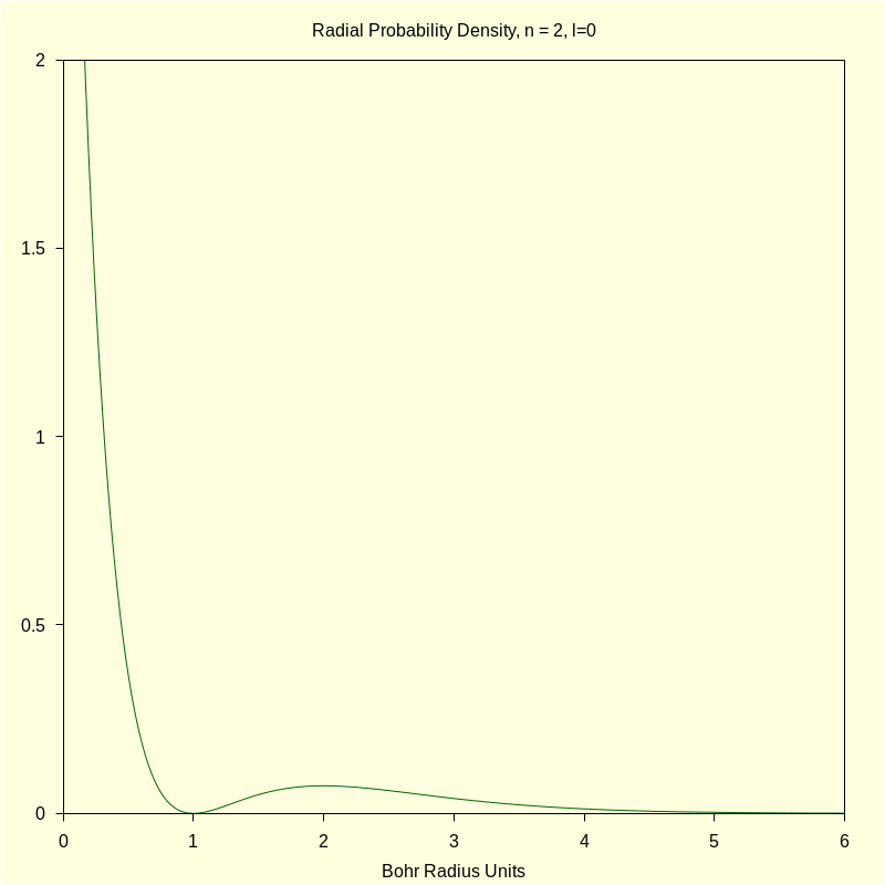
The angular probability density is constant for this orbital, but since n=2 there will be some radial modulation of the total density as shown in the following radial plot.

4.1.2 Radial Probability Density

-->	wxdraw2d ( proportional_axes = none , color = dark_green , explicit ( rprob , r , 0 , 6 ) , title = "Radial Probability Density, n = 2" , ytics = true , xrange = [ 0 , 6 ] , yrange = [ 0 , 2 ] ) $

\[\operatorname{ }\]

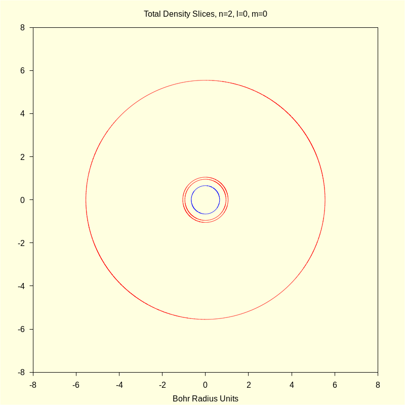
Note that as the radial distance increases, the probability actually falls to zero and then rises again (due to the radial polynomial factor) before falling toward zero ultimately (due to the radial exponential factor). This is charcteristic of all radial density functions.

4.1.3 Total Density "Slices"

We now combine the two probability densities (i.e. R(r) * Y(θ, φ)) by plotting several contours of this total density function at a fixed value of φ.

-->

p1 : 1e-2 $ p2 : 1e-4 $
wxdraw2d ( color = blue , proportional_axes = xy ,
implicit ( rprob ( sqrt ( x ^ 2 + y ^ 2 ) ) · aprob ( atan2 ( x , y ) , 0 ) − p1 , x , − 8 , 8 , y , − 8 , 8 ) ,
color = red , implicit ( rprob ( sqrt ( x ^ 2 + y ^ 2 ) ) · aprob ( atan2 ( x , y ) , 0 ) − p2 , x , − 8 , 8 , y , − 8 , 8 ) ) $

Note how at a high density value (blue) there is only a single contour "slice". This corresponds to the single intersection with the radial density curve, near 1 Bohr radius, as can be seen in the previous plot. For lower values of radial density (red) there are three intersections which form the three contour "slices."

4.1.4 Total Density Contour Surface

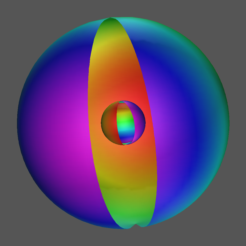
Finally, at a selected value of the total density (from the red value in previous image), we form the surface of revolution. The two outermost spheres are "sliced" open to reveal the interiors. The innermost sphere is not sliced. The coloration of the spheres is used only to provide contrast and has no relation to the complex phase. To better view, and appreciate, the totality of this atomic orbital an animation is provided that will zoom in toward the center. Click on the image or link to view the Ogg format video.

Click Image for Video

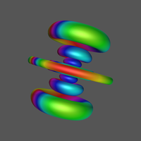
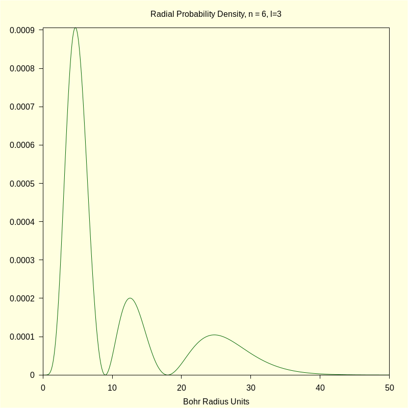
It is critical to understand that this surface does not represent the actual AO. Rather it is only a 3-D "slice" of the 4-D structure. The actual AO is composed of an infinite series of such "slices" outward to infinity with each "slice" being a particular value of probability. We can perhaps liken it to a block of solid material that contains variations in density or temperature throughout. In the case of AOs the material is space and the variations are of probability.

4.2 Quantum Numbers n=6, l=3, and m=1.

Let us now apply the above concepts and methods to a much more complicated AO with n=6, l=3, and m=1. All we need do is plug in the quantum numbers and Maxima does the rest.

This orbital has the physical designation ψ_631.

-->	kill ( all ) $

-->

n : 6 $ l : 3 $ m : 1 $
coeff : %i ^ ( m + abs ( m ) ) · sqrt ( ( ( l − abs ( m ) ) ! ) / ( ( l + abs ( m ) ) ! ) ) · sqrt ( ( 2 · l + 1 ) / 4 / %pi ) $
P_lm : expand ( assoc_legendre_p ( l , abs ( m ) , cos ( θ ) ) ) $
define ( aprob ( θ , φ ) , ( coeff · P_lm ) ^ 2 ) ;
/* calculate radial probability */
a : n − l − 1 $ b : 2 · l + 1 $ ρ : 4 / n $
L : expand ( sum ( ( ( a + b ) ! ) / ( ( k + b ) ! ) / ( ( a − k ) ! ) / ( k ! ) · ( − r · ρ ) ^ k , k , 0 , a ) · ρ ^ l · r ^ l ) $
Rcoeff : ρ ^ ( 3 / 2 ) · sqrt ( ( ( n − l − 1 ) ! ) / ( 2 · n ) / ( ( n + l ) ! ) ) · exp ( − ρ · r / 2 ) $
define ( rprob ( r ) , ( L · Rcoeff ) ^ 2 ) ;

\[\operatorname{ }\operatorname{aprob}\left( \theta \operatorname{,}\phi \right) \operatorname{:=}\frac{7 {{\left( \frac{3 \sqrt{1-{{\cos{\left( \theta \right) }}^{2}}}}{2}-\frac{15 {{\cos{\left( \theta \right) }}^{2}} \sqrt{1-{{\cos{\left( \theta \right) }}^{2}}}}{2}\right) }^{2}}}{48 \pi }\]

\[\operatorname{ }\operatorname{rprob}(r)\operatorname{:=}\frac{{{\left( \frac{16 {{r}^{5}}}{243}-\frac{16 {{r}^{4}}}{9}+\frac{32 {{r}^{3}}}{3}\right) }^{2}} {{e}^{-\frac{2 r}{3}}}}{7348320}\]

-->

\[\operatorname{ }\frac{\int_{0}^{\infty }{\left. {{r}^{2}} {{\left( \frac{16 {{r}^{5}}}{243}-\frac{16 {{r}^{4}}}{9}+\frac{32 {{r}^{3}}}{3}\right) }^{2}} {{e}^{-\frac{2 r}{3}}}dr\right.}}{7348320}\]

\[\operatorname{ }1\]

\[\operatorname{ }\int_{0}^{2 \ensuremath{\pi} }{\left. \frac{7 \int_{0}^{\ensuremath{\pi} }{\left. {{\left( \frac{3 \sqrt{1-{{\cos{\left( \theta \right) }}^{2}}}}{2}-\frac{15 {{\cos{\left( \theta \right) }}^{2}} \sqrt{1-{{\cos{\left( \theta \right) }}^{2}}}}{2}\right) }^{2}} \sin{\left( \theta \right) }d\theta \right.}}{48 \ensuremath{\pi} }d\phi \right.}\]

\[\operatorname{ }1\]

4.2.1 Angular Probability Density

Geomview with StageTools produces the following plot given the above equation. The coloration is aligned with the z-axis and has no relation to the complex phase.

To fully appreciate the shape of this angular density be sure to view the Ogg format video by clicking the link.

Click Image for Video

4.2.2 Radial Probability Density

The 3rd degree polynomial factor produces two nodes in the radial distribution and this leads to more complicated orbital shapes.

-->	wxdraw2d ( proportional_axes = none , color = dark_green , explicit ( rprob , r , 0 , 50 ) , title = "Radial Probability Density, n = 6" ) $

\[\operatorname{ }\]

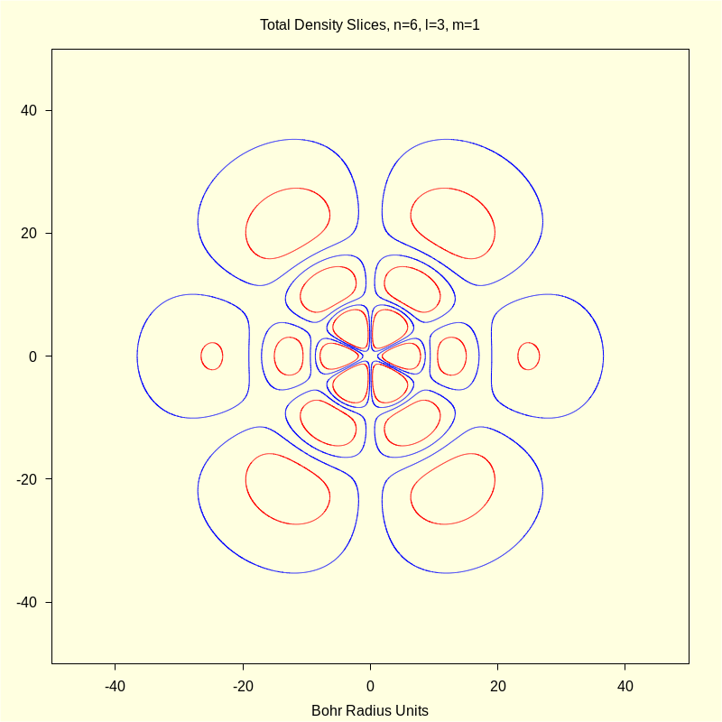
4.2.3 Total Density "Slices"

Choosing two different values for the total probability density, we now plot two separate contour "slices" of the combined radial and angular densities. The rather extreme modulation of the angular density by the radial density is quite apparent.

-->	p1 : 1e-6 $ p2 : 1e-5 $ wxdraw2d ( color = blue , implicit ( rprob ( sqrt ( x ^ 2 + y ^ 2 ) ) · aprob ( atan2 ( x , y ) , 0 ) − p1 , x , − 50 , 50 , y , − 50 , 50 ) , color = red , implicit ( rprob ( sqrt ( x ^ 2 + y ^ 2 ) ) · aprob ( atan2 ( x , y ) , 0 ) − p2 , x , − 50 , 50 , y , − 50 , 50 ) ) ;

\[\operatorname{ }\]

Using a single value for the total density (corresponding to the red color in the above plot) we create the surface of revolution and display it with Geomview. Be sure to view the accompanying Ogg video to fully discern the complex orbital shape. Also to note is that the coloration in this case does correspond to the complex phase.

Click Image for Video

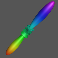
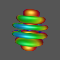
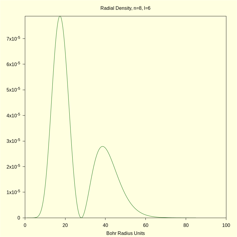
4.3 Quantum Numbers n=8, l=6, and m=1.

Let's now proceed to an even higher level with n=8, l=6, m=1. This comparatively very high energy level is seldom depicted in other AO visual material. But with GNU/Linux and Maxima the visualization becomes routine.

This orbital, or linear combinations thereof, is sometimes called the "i" orbital but the precise designation is Ψ_861.

(%i15)

n : 8 $ l : 6 $ m : 1 $
/* calculate angular probability */
Acoeff : %i ^ ( m + abs ( m ) ) · sqrt ( ( ( l − abs ( m ) ) ! ) / ( ( l + abs ( m ) ) ! ) ) · sqrt ( ( 2 · l + 1 ) / 4 / %pi ) $
P_lm : expand ( assoc_legendre_p ( l , abs ( m ) , cos ( θ ) ) ) $
define ( aprob ( θ , φ ) , trigreduce ( ( Acoeff · P_lm ) ^ 2 ) ) ;
/* calculate radial probability */
a : n − l − 1 $ b : 2 · l + 1 $ ρ : 4 / n $
L : expand ( sum ( ( ( a + b ) ! ) / ( ( k + b ) ! ) / ( ( a − k ) ! ) / ( k ! ) · ( − r · ρ ) ^ k , k , 0 , a ) · ρ ^ l · r ^ l ) $
Rcoeff : ρ ^ ( 3 / 2 ) · sqrt ( ( ( n − l − 1 ) ! ) / ( 2 · n ) / ( ( n + l ) ! ) ) · exp ( − ρ · r / 2 ) $
define ( rprob ( r ) , ( L · Rcoeff ) ^ 2 ) ;

\[\operatorname{ }\operatorname{aprob}\left( \theta \operatorname{,}\phi \right) \operatorname{:=}\frac{-297297 \cos{\left( 12 \theta \right) }-216216 \cos{\left( 10 \theta \right) }-129402 \cos{\left( 8 \theta \right) }-32760 \cos{\left( 6 \theta \right) }+83265 \cos{\left( 4 \theta \right) }+248976 \cos{\left( 2 \theta \right) }+343434}{1048576 \ensuremath{\pi} }\]

\[\operatorname{ }\operatorname{rprob}(r)\operatorname{:=}\frac{{{\left( \frac{7 {{r}^{6}}}{32}-\frac{{{r}^{7}}}{128}\right) }^{2}} {{e}^{-\frac{r}{2}}}}{11158821273600}\]

(%i30)

/* check for normalization */
' integrate ( rprob ( r ) · r ^ 2 , r , 0 , inf ) ; integrate ( rprob ( r ) · r ^ 2 , r , 0 , inf ) ;
' ( integrate ( ' integrate ( aprob ( θ , φ ) · sin ( θ ) , θ , 0 , %pi ) , φ , 0 , 2 · %pi ) ) ;
integrate ( integrate ( aprob ( θ , φ ) · sin ( θ ) , θ , 0 , %pi ) , φ , 0 , 2 · %pi ) ;

\[\operatorname{ }\frac{\int_{0}^{\infty }{\left. {{r}^{2}} {{\left( \frac{7 {{r}^{6}}}{32}-\frac{{{r}^{7}}}{128}\right) }^{2}} {{e}^{-\frac{r}{2}}}dr\right.}}{11158821273600}\]

\[\operatorname{ }1\]

\[\operatorname{ }\int_{0}^{2 \ensuremath{\pi} }{\left. \int_{0}^{\ensuremath{\pi} }{\left. \sin{\left( \theta \right) } \operatorname{aprob}\left( \theta \operatorname{,}\phi \right) d\theta \right.}d\phi \right.}\]

\[\operatorname{ }1\]

4.3.1 Angular Probability Density

Again, Geomview with StageTools produces the following plot given the above angular density equation. The coloration is aligned with the z-axis to better allow visualization and has no relation to the complex phase (which is not terribly relevant).

To fully appreciate the shape of this angular density be sure to view the Ogg format video by clicking the image or link.

Click Image for Video

4.3.2 Radial Probability Density

(%i34)

wxdraw2d ( proportional_axes = none , color = dark_green , explicit ( rprob , r , 0 , 100 ) ,
title = "Radial Density, n=8, l=6" , xlabel = "Bohr Radius Units" ) $

\[\operatorname{ }\]

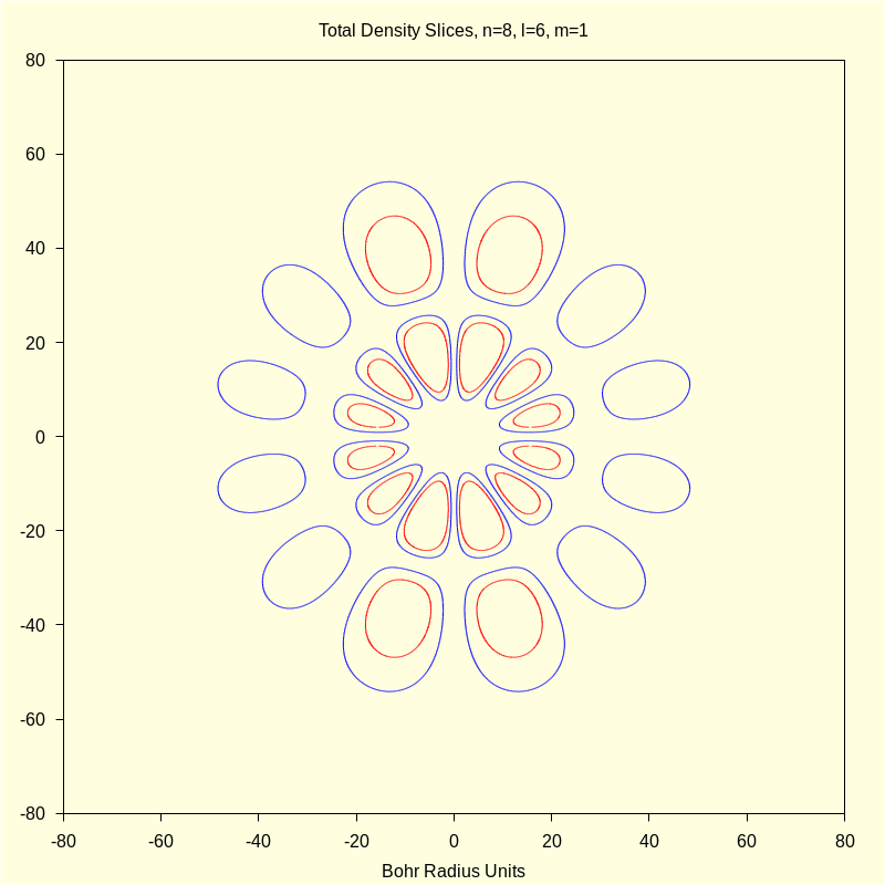
4.3.3 Total Density "Slices"

The total density contour "slices" for two different values of probability.

(%i37)

p1 : 1e-6 $ p2 : 4e-6 $
wxdraw2d ( color = blue , implicit ( rprob ( sqrt ( x ^ 2 + y ^ 2 ) ) · aprob ( atan2 ( x , y ) , 0 ) − p1 , x , − 80 , 80 , y , − 80 , 80 ) ,
color = red , implicit ( rprob ( sqrt ( x ^ 2 + y ^ 2 ) ) · aprob ( atan2 ( x , y ) , 0 ) − p2 , x , − 50 , 50 , y , − 50 , 50 ) ,
title = "Total Density Slices, n=8, l=6, m=1" , xlabel = "Bohr Radius Units" ) $

Again, using a single value for the total density (corresponding to the blue color in the above plot) we create the surface of revolution and display it with Geomview. Be sure to view the accompanying Ogg video to fully discern the complex orbital shape. Also to note is that the coloration in this case does correspond to the complex phase.

The video has a slight but still noticeable "stutter" due to the extreme amount of computation performed by Geomview at each increment of the rotation.

Click Image for Video

5 Epilogue

This article demonstrates the ease with which even very high energy atomic orbital functions can be derived and plotted by using Maxima/wxMaxima. Atomic orbitals with any set of quantum numbers can be produced at will. There is no need to consult reference books, and most references do not include AOs beyond n=6.

As a supplement, the graphic utilities of Geomview can produce stunning output and coupled with StageTools and ffmpeg AO videos can be realized.

As always, the interested reader is encouraged to explore these, and other, GNU/Linux tools.

Created with wxMaxima.
Modified and embedded by L.A.P.